To Stabilize the Debt, Policymakers Should Seek Another $1.4 Trillion in Deficit Savings
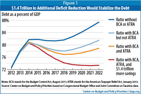
With the “fiscal cliff” deal in place, President Obama and Congress are now expected to seek more deficit reduction to replace the automatic spending cuts (“sequestration”) that are scheduled to take effect on March 1. Policymakers can stabilize the public debt over the coming decade, ensuring that it doesn’t grow faster than the economy and risk eventual economic problems, with $1.4 trillion in additional deficit savings over the next decade (see Box 2). Policymakers can achieve the $1.4 trillion with $1.2 trillion in policy savings — tax increases and spending cuts — because that would generate almost $200 billion in savings in interest payments. That $1.4 trillion in deficit savings would stabilize the debt at about 73 percent of Gross Domestic Product (GDP) over the latter part of the decade (see Figure 1).[1]
That $1.4 trillion — and not a larger amount — would stabilize the debt is due primarily to the deficit-reduction policies that the President and Congress have enacted over the last two years. First came $1.5 trillion in appropriations cuts (and another $200 billion in associated interest savings), primarily through the annual caps in the 2011 Budget Control Act (BCA).[2] Second came the tax increases in the fiscal cliff deal, officially called the American Taxpayer Relief Act (ATRA).
In addition, the Congressional Budget Office’s (CBO) revised economic and budget projections in August 2012 show a more sanguine outlook for the coming decade than its earlier projections. Those updated projections reduced estimated deficits under current policies by about $750 billion over the coming decade, relative to CBO’s March 2012 baseline, and by about $1.5 trillion relative to its August 2010 forecast, which the Bowles-Simpson and Rivlin-Domenici commissions used for their reports of late 2010.
That baseline, with those assumptions, is consistent with the baselines of other budget analysts. Like us, the Obama Administration, the Bowles-Simpson commission, the Rivlin-Domenici commission, the Bipartisan Policy Center (BPC), and the Committee for a Responsible Federal Budget (CRFB) all have used baselines which assume that policymakers will offset the costs of continuing the tax extenders and will not offset the cost of blocking the Medicare physician cuts. Also like us, the BPC and CRFB both assumed that policymakers will cancel “sequestration” without offsetting the cost (and the Bowles-Simpson and Rivlin-Domenici commissions issued their reports before policymakers created “sequestration”).
Needless to say, the amount of deficit reduction needed to stabilize the debt will rise or fall if these assumptions change (see Appendix II). If, for instance, one assumes that policymakers will let the “sequestration” take effect, then they would have to find only an additional $257 billion in deficit savings to stabilize the debt. Or, if, conversely one assumes that policymakers will not offset the costs of continuing the tax extenders, they would have to find another $1.8 trillion in deficit reduction to stabilize the debt. In some respects, this $1.8 trillion estimate reflects a worst-case scenario, because it assumes not only that policymakers will continue the tax extenders without paying for them, but that (consistent with our underlying baseline assumptions) they cancel sequestration without putting anything in its place and cancel the scheduled cuts in Medicare reimbursements for doctors without paying for them.
Box 1: All Figures Will Change When CBO Issues Its New Baseline
All the figures in this analysis will change when CBO issues its new baseline in a few weeks. There are two reasons.
First, the "ten-year budget window" commonly used by budget analysts will change: it now covers 2013-2022 but will soon cover 2014-2023. By itself, this will increase the needed policy savings by about $200 billion because we will be counting another year of the savings, 2023. But this will add little or no difficulty to the task; if policymakers can find $1.2 trillion in policy savings through 2022, a simple continuation of those polices will almost surely yield the required additional $200 billion in 2023.
Second, CBO will also change its underlying economic and technical budget forecast from the one it most recently issued in August 2012, whose estimates underlie this report. By themselves, new CBO estimates could make the challenge hundreds of billions of dollars easier or harder, and at this point we don’t know which.
| Table 1 Deficit Reduction to Stabilize the Debt (cumulative totals, 2013-2022, in billions) | |||
| Policy savings | Interest savings | Total deficit reduction | |
| Discretionary savings from cuts in 2011 funding and caps imposed by the BCA | 1,465 | 236 | 1,701 |
| Savings from the ATRA | 566 | 81 | 647 |
| Further savings needed to stabilize debt | 1,191 | 177 | 1,368 |
| TOTAL | 3,223 | 493 | 3,716 |
| Notes: BCA stands for the Budget Control Act, August 2011; ATRA stands for the American Taxpayer Relief Act, January 2013; all savings measured relative to current policy (see Appendix I) Source: Center on Budget and Policy Priorities based on Congressional Budget Office and Joint Committee on Taxation data. | |||
Policymakers, of course, would have to decide how to achieve the $1.4 trillion in deficit savings —specifically, what changes to make in tax and spending policies in order to generate $1.2 trillion in policy savings (and the $200 billion in interest savings that would come with it). Even if they split the $1.2 trillion evenly between tax increases and program cuts, however, the total savings enacted since 2011 would consist of almost $2 in program cuts for every $1 in revenues. That’s because most of the policy savings that policymakers have achieved so far have occurred on the spending side, even after taking ATRA into account.
This $1.4 trillion in additional deficit reduction would, when combined with the appropriations cuts of 2011 and the savings from ATRA, produce a total of $3.7 trillion in deficit reduction (see Table 1). The resulting three-part package would (based on savings in the fifth year as a percentage of GDP) be as large as the 1990 deficit-reduction agreement and larger than the 1993 agreement — the two big budget deals that played an important role in converting the large deficits of the early 1990s to four years of budget surpluses that began in 1998.
| Table 2 Revenue Increases vs. Program Cuts (cumulative totals, 2013-2022, in billions) | ||||
| Program cuts | Revenue increases | Interest savings | TOTAL | |
| Discretionary savings from cuts in 2011 funding and BCA | 1,465 | 0 | 236 | 1,701 |
| Savings from the ATRA | 3 | 563 | 81 | 647 |
| TOTAL enacted savings to date | 1,468 | 563 | 317 | 2,348 |
| Share of savings | 72% | 28% | ||
| Scenario A: All further savings come from program cuts | 1,191 | 0 | 177 | 1,368 |
| TOTAL savings (including those previously enacted) | 2,659 | 563 | 493 | 3,716 |
| Share of savings | 83% | 17% | ||
| Scenario B: Further savings come equally from program cuts and revenue increases | 596 | 596 | 177 | 1,368 |
| TOTAL savings (including those previously enacted) | 2,064 | 1,159 | 493 | 3,716 |
| Share of savings | 64% | 36% | ||
| Scenario C: All further savings come from revenue increases | 0 | 1,191 | 177 | 1,368 |
| TOTAL savings (including those previously enacted) | 1,468 | 1,754 | 493 | 3,716 |
| Share of savings | 46% | 54% | ||
| Notes: may not add due to rounding; BCA stands for the Budget Control Act, August 2011; ATRA stands for the American Taxpayer Relief Act, January 2013; all savings measured relative to current policy (see Appendix I) Source: Center on Budget and Policy Priorities based on Congressional Budget Office and Joint Committee on Taxation data. | ||||
Overall, Program Cuts Would Outweigh Revenue Increases Even if Additional Savings Are Split Equally
The majority of the policy savings that policymakers have achieved so far, starting with cuts in 2011 funding, have occurred on the spending side. As Table 2 shows, about $2.0 trillion of policy savings (excluding interest savings) have been enacted to date, of which $1.5 trillion or 72 percent reflects program cuts and $0.6 trillion or 28 percent reflects new revenue.[4]
Table 2 presents three different scenarios for achieving the $1.2 trillion of additional policy savings needed to stabilize the debt: Scenario A assumes all of the additional savings come from program cuts; Scenario B assumes the savings are evenly divided between program cuts and revenue increases; and Scenario C assumes that all of the savings come from higher revenues.
As Scenario B shows, even if the additional savings were divided evenly between revenue increases and program cuts, the total deficit reduction under the three deficit-reduction packages would be heavily weighted toward budget cuts: 64 percent budget cuts to 36 percent revenue increases, or a ratio of nearly 2 to 1. To achieve a 50-50 split for the combined deficit-reduction packages, policymakers would have to obtain nearly 90 percent of the additional $1.2 trillion in savings from revenue increases.[5]
In contrast, if all of the additional savings were to come from program cuts, as Republican congressional leaders have suggested, the overall ratio would be still more skewed, with more than four-fifths coming on the spending side — a ratio of nearly 5 to 1.
Health Care Costs Pose Significant Longer-Term Challenge
Though it would stabilize the debt over the coming decade, an additional $1.4 trillion in deficit reduction would not be enough to address the longer-term budget problem. In ensuing decades, the aging of America’s population and projected increases in per-capita health care costs — which are likely to rise faster than per-capita GDP — will put considerable pressure on federal health and retirement programs, returning the budget to an unsustainable path of rising debt as a share of the economy. Nevertheless, by stabilizing the debt for the next decade, an additional $1.4 trillion in deficit savings would give experts and policymakers time to figure out how to slow the growth of health care costs throughout the U.S. health care system without impairing the quality of care.
There are major unknowns in the health arena. The growth of both public and private health costs has slowed appreciably in the past few years; spending for Medicare — the largest federal health program — grew by only 3.2 percent in fiscal year 2012, CBO has reported,[6] as compared with average growth of 6.7 percent a year from 2007 through 2011. CBO’s latest projections of total Medicare spending under current policy over the coming decade are about $400 billion below the projections CBO made just two years ago. Experts don’t yet know whether this slowdown is permanent, generating even more savings than CBO has projected to date, or only temporary as CBO assumes. The answer will affect both the magnitude of the long-term fiscal problem and the extent to which further slowing of health-care cost growth is required.
More fundamentally, we currently lack needed information on how to slow health cost growth without reducing health care quality or impeding access to needed care. Demonstration projects and other experiments to find ways to do so are now starting, some of them government-funded and others being undertaken in the private sector. By later in the decade, we should have substantially more knowledge of what works and what doesn’t. Taking major policy action in this area now, before we have the necessary knowledge and experience, risks putting us on a course that could fail to restrain health costs, compromise health care quality, or harm substantial numbers of sick or otherwise vulnerable individuals. An additional $1.4 trillion in deficit reduction would, by stabilizing the debt for the coming decade, buy time to find answers to these important questions.
Box 2: Why the Debt Ratio Matters
The debt ratio — the debt held by the public as a share of GDP — should rise only during hard times or major emergencies and should fall during good times. That allows the ratio to remain stable over the business cycle as a whole and enables the government to combat recessions through tax cuts and spending increases (and to address human misery during bad times).
The debt ratio cannot rise forever. If it did, that would shrink the amount of national saving available for private investment, ultimately impairing productivity growth and, in turn, living standards. Alternatively, if foreign capital offsets the shortfall in domestic capital, the profits from that investment will go abroad; either way, U.S. living standards would suffer. In a crisis, international credit markets might refuse to lend to the U.S. public or private sectors at a reasonable price. These problems would occur if the debt ratio became too high. While no one knows what “too high” means for the United States, a debt ratio that rises in both good times and bad will become increasingly problematic.
That’s why the minimum appropriate budget policy is to ensure that the debt ratio does not rise during normal economic times. Achieving that would require shrinking deficits to below 3 percent of GDP. In the illustrative debt path that includes the additional $1.4 trillion of deficit reduction shown in Figure 1, deficits average 2.5 percent of GDP from 2018 through 2022.
Achieving $1.4 trillion in additional deficit savings would stabilize the debt at about 73 percent of GDP by 2018. Some analysts prefer a lower debt ratio, such as 60 percent of GDP, a goal that the European Union and the International Monetary Fund adopted some years ago. No economic evidence supports this — or any other — specific target, however, and IMF staff have made clear that the 60 percent criterion is an arbitrary one. In addition, even if such a target were the best one before the recent severe economic downturn pushed up debt substantially in most advanced countries, it would not necessarily be an appropriate target for debt over the next ten years, given the severity of the downturn and continued economic weakness. The critical goal now is to stabilize the debt in the coming decade.
Stabilizing the debt during this decade will not permanently solve our fiscal problems; policymakers will need to enact additional deficit reduction for the long term. But it would represent an important accomplishment.
It also should be noted that there can be risks in policymakers setting their sights too high. If the political obstacles facing a much larger deficit-reduction package are too great, then insistence on a package that goes well beyond stabilizing the debt could lead either to failure — i.e., to enactment of no deficit-reduction package — or to a package that provides false security because it is dominated by budget gimmicks that don’t actually reduce our long-term deficits but merely appear to do so. ATRA already contains one such gimmick.*
*The $12 billion in revenue “increases” in ATRA is actually the result of a large timing shift created by an additional tax giveaway that will primarily benefit affluent households. See Robert Greenstein, “Budget Deal Gives New Tax Cut to the Wealthy ? and Pretends It's a Tax Increase,” Off the Charts blog, January 2, 2013,
Appendix I:
Current Policy and Methodology
Current policy. We described the concepts underlying our current-policy baseline on November 1, 2012, when we first calculated that $2 trillion in additional deficit reduction (including interest savings) was needed to stabilize the debt ratio by the second half of the decade. Appendix I of that analysis (cited in footnote 1) explains the detailed concepts behind that baseline. For consistency with that analysis and analyses previously published by the Bipartisan Policy Center and the Committee for a Responsible Federal Budget, we continue to use those baseline concepts in this analysis. Broadly, our current-policy baseline assumes that: the 2001/2003/2009 tax cuts will be continued indefinitely; those normal tax extenders that are continued will be paid for; relief from scheduled cuts in reimbursements to Medicare physicians will be granted on an ongoing basis without the costs being offset, and the sequestration scheduled to occur on January 2, 2013 (and now postponed by ATRA) will be entirely cancelled (again, without the costs being offset).[7]
Our estimate of the $566 billion in savings associated with ATRA comes from CBO’s cost estimate issued January 1, 2013. CBO’s cost estimate looks different from our figure because CBO measures revenue changes relative to current law rather than current policy. Relative to current law, the continuation of the 2001/2003/2009 tax cuts is a cost, but relative to current policy, the fact that some of the tax cuts for the very wealthy have ended results in savings.
Both we and CBO treat ATRA’s temporary continuation of certain “normal tax extenders” as a cost (but we do not treat the continuation of Section 179 expensing as a cost because we view that provision of the tax code as part of the 2001/2003/2009 tax cuts and so our baseline already assumed that it would be continued). Unlike CBO, we do not treat the temporary extension of Sustainable Growth Rate relief for Medicare physicians as a cost because our baseline already assumed that it would be continued. CBO treats the $24 billion reduction in the scheduled sequestration as a cost relative to current law (which assumes the sequestration would take effect), but we do not treat it as a cost because our current-policy baseline assumes the sequestration would be cancelled and so already reflects those costs.
Method for modeling hypothetical deficit reduction. Relative to the current-policy baseline described above, as modified by ATRA, we build a hypothetical deficit-reduction path. We assume that deficit reduction will start in fiscal year 2014 and be fully phased in by 2016. We select a dollar amount of policy savings for 2014 and assume it will double in 2015, triple in 2016, and grow in nominal terms by 6.7 percent per year thereafter. We choose 6.7 percent because that is the un-weighted average annual growth rate of revenues and Medicare in the current-policy baseline. To the extent that the bulk of additional deficit reduction comes from revenues and health entitlements, it is reasonable to expect that, once the policies in question are fully phased in, the savings will grow at the same rate as the baselines of these programs. Finally, we use CBO’s August 2012 interest rates to calculate the interest savings that will occur as a result of the policy savings we assume.
More precisely, given a target for total deficit reduction over ten years, we sought a starting figure for policy savings in 2014 that produces the desired ten-year total results. Table 3 shows the year-by-year policy and interest savings associated with the hypothetical $1.4 trillion deficit-reduction path used in this analysis.
| Table 3 Policy Savings and Interest Savings in the Hypothetical $1.4 Trillion Path In billions of dollars | |||
| Fiscal year | Policy savings | Interest savings | Total savings |
| 2013 | 0 | 0 | 0 |
| 2014 | 41 | O | 41 |
| 2015 | 83 | 1 | 84 |
| 2016 | 124 | 3 | 127 |
| 2017 | 133 | 8 | 140 |
| 2018 | 142 | 16 | 157 |
| 2019 | 151 | 24 | 175 |
| 2020 | 161 | 32 | 194 |
| 2021 | 172 | 41 | 214 |
| 2022 | 185 | 51 | 235 |
| Total | 1,191 | 177 | 1,368 |
| May not add due to rounding | |||
Finally, in calculating the resulting debt as a percent of GDP and displaying it in Figure 1, we smooth the path of deficits and debt to avoid certain meaningless bumps in the path. Four programs (SSI, veterans’ compensation and pensions, military retirement, and Medicare payments to Medicare Advantage and Part D plans) include a provision whereby, if the scheduled monthly payment would fall on a weekend, it is accelerated to the prior Friday. When October 1 (the first day of the fiscal year) falls on a weekend, the payment normally made on that date instead occurs on September 29 or 30, which is in the prior fiscal year. As a result, while most fiscal years include 12 such monthly payments, a few include 11 or 13. This makes deficit and debt figures appear bumpier than they really are (and happens to overstate the deficit and debt in 2022 by $44 billion because that year includes 13 such monthly payments). To make the resulting debt levels and path more meaningful, we assume 12 monthly payments in each fiscal year. We build this assumption into the current-policy baseline so that this smoothing does not count as deficit reduction or a deficit increase.
Appendix II:
Alternative Approaches to Current Policy
As discussed in Appendix I, the current-policy baseline used in this analysis makes a number of important assumptions. This appendix examines in more detail the effect of employing different assumptions with regard to the tax extenders and the sequestration.
Tax extenders. Congress generally extends a large series of special tax provisions, generally relating to the treatment of business income, for a year or two at a time. The Research and Experimentation tax credit is the most prominent. ATRA extended many of these special provisions until December 31, 2013.
We do not assume their continuation in this current-policy baseline beyond what was provided in ATRA largely because the Bowles-Simpson commission and the Obama Administration, in its 2013 budget, did not continue them in their current-policy baselines. The Bipartisan Policy Center and the Committee for a Responsible Federal Budget have adopted the same approach in their current-policy baselines. We think it will be less confusing if we maintain broad comparability with their baselines.
There is a good case, however, for treating the normal tax extenders (NTEs) like any other expiring tax provision that was intended to be permanent. What if we had used a current-policy baseline in which the NTEs were assumed to be continued?
Under such a baseline, the starting level of post-ATRA tax expenditures would be $365 billion higher (and thus revenues lower) over the period 2013-2022, reflecting the continuation of all the NTEs. (We assume that the NTEs do not include the 50 percent deduction for the cost of certain new capital investments known as “bonus depreciation,” which was enacted to address the slowdown in the economy and which we expect will not be extended once the economy is on more solid ground. During the recession in the early 2000s, a similar depreciation provision was allowed to expire when the economy had recovered.) When the associated interest costs of $51 billion are included, then the current-policy baseline deficit would be $416 billion higher over ten years if the extension of the NTEs were included. [8] Consequently, stabilizing the debt would require $1.8 trillion, not $1.4 trillion, in deficit reduction, including interest savings. By the same token, however, one could achieve the “extra” needed deficit reduction by allowing the NTEs to expire or paying for those NTEs that policymakers choose to extend.
In short, you get to the same bottom line if you start with a baseline in which the NTEs have expired and then find $1.4 trillion in deficit reduction, or if you start with a baseline in which the NTEs are continued and then find $1.8 trillion in deficit reduction, of which up to $416 billion could be achieved by the expiration of some or all of the NTEs or by paying for those NTEs you chose to continue.[9] The resulting levels of revenues and debt are the same either way.
Sequestration. The current-policy baseline used in this analysis does not reflect the implementation of sequestration, or automatic across-the-board spending cuts, required under the Budget Control Act (BCA). The BCA established a congressional Joint Select Committee on Deficit Reduction (the “supercommittee”) to develop legislation to reduce deficits by $1.2 trillion over ten years and created the sequestration as a backup mechanism to achieve this deficit reduction in the event the supercommittee failed.
If the current-policy baseline assumed instead that the sequestration went into effect, it would produce $948 billion of savings through budget cuts over the ten years 2013 to 2022, and $163 billion of associated interest savings. This yields total deficit reduction of $1.1 trillion over the decade.[10] Consequently, stabilizing the debt would require only $257 billion, not $1.4 trillion, in additional deficit reduction, including interest savings.
The key point of both of these examples is that everyone — policymakers, the media, the public, and the business community — must be aware of what is in the baseline. If the baseline assumes the expiration of the NTEs (as ours does), then policymakers cannot count the expiration of any NTEs as deficit reduction, and they must count as a cost the extension of any NTEs that aren’t paid for. Similarly, if the baseline assumes the sequestration is not implemented (as ours does), then policymakers would count the replacement of the sequestration with other savings as deficit reduction, but would not count as a cost rolling back the sequestration without offsets.
End Notes
[1] This analysis updates our previous report on the subject to reflect the enactment of the American Taxpayer Relief Act (ATRA). The previous report included more extensive discussion of the points made in this report; see Richard Kogan, $2 Trillion in Deficit Savings Would Achieve Key Goal: Stabilizing the Debt over the Next Decade, Center on Budget and Policy Priorities, November 1, 2012, https://www.cbpp.org/cms/index.cfm?fa=view&id=3856. Because ATRA reduces projected deficits by more than $0.6 trillion, the additional deficit reduction needed to stabilize the debt shrinks from the $2 trillion discussed in the previous report to almost $1.4 trillion, as shown in this report.
[2] Under those caps, discretionary spending over 2013-2022 will be $1.5 trillion below the levels in the Congressional Budget Office (CBO) baseline from the end of 2010, when the Bowles-Simpson and Rivlin-Domenici commissions issued their plans, according to CBO estimates. See Richard Kogan, Congress Has Cut Discretionary Funding by $1.5 Trillion over Ten Years, Center on Budget and Policy Priorities,September 25, 2012, https://www.cbpp.org/cms/index.cfm?fa=view&id=3840.
[3] This reflects the cost of continuing all of the normal tax extenders, except for the “bonus depreciation” provision in ATRA that allows companies to write off 50 percent of the cost of new equipment. We assume that provision will be allowed to expire once the economy is stronger, as was the case when a similar provision was enacted during the recession of the early 2000s. See Appendix II.
[4] The revenue raised in ATRA shown in Table 2 is $563 billion. This total reflects $624 billion from raising taxes on certain upper-income households by allowing certain provisions enacted in 2001 and 2003 to expire at the end of 2012, net of the effects of other provisions in the bill, primarily the temporary continuation of the so-called “tax extenders.”
[5] For more on why all the steps in a deficit reduction journey should be taken into account, see Richard Kogan, “Of Zeno’s Dichotomy Paradox, ‘Takers,’ and Deficit Reduction,” Off the Charts blog, February 16, 2012, http://www.offthechartsblog.org/of-zenos-dichotomy-paradox-takers-and-deficit-reduction/.
[6] This figure subtracts premiums paid by beneficiaries and corrects for shifts in the timing of payments. Congressional Budget Office, Monthly Budget Review, Fiscal Year 2012, October 5, 2012, http://www.cbo.gov/sites/default/files/cbofiles/attachments/2012_09_MBR.pdf.
[7] We calculated the levels of spending, revenues, and deficits in that current-policy baseline from estimates CBO issued in August 2012, except that the cost of certain tax continuations was modified very slightly to reflect new estimates published by the Joint Committee on Taxation in December 2012.
[8] In our November 1, 2012 report, we stated that the continuation of NTEs would increase the deficit by about $1 trillion. We have revised this figure to $416 billion for several reasons. First, as explained above, we no longer consider bonus depreciation an NTE, which reduces the revenue loss of NTEs by $341 billion over ten years. Second, ATRA did not extend certain tax expenditures that expired in 2011 and 2012, and therefore we no longer consider them NTEs; these tax expenditures would have reduced revenues by $73 billion over ten years. Third, the temporary extension of NTEs in ATRA reduced revenues by $69 billion over ten years; this cost is now built into our current-policy baseline rather than in the estimate of extending the NTEs. Finally, given the smaller revenue loss from continuing the NTEs, the associated interest costs are about $100 billion lower over ten years. See Richard Kogan, “$2 Trillion in Deficit Savings Would Achieve Key Goal: Stabilizing the Debt Over the Next Decade,” Center on Budget and Policy Priorities, November 1, 2012, https://www.cbpp.org/cms/index.cfm?fa=view&id=3856.
[9] On August 1, 2012, CRFB issued a statement strongly urging Congress to offset the cost of any of the NTEs it does continue. See http://crfb.org/sites/default/files/Dont_Put_the_Extenders_on_the_Nations_Credit_Card.pdf.
[10] Note that the $1.1 trillion in deficit reduction is less than the $1.2 trillion sequestration targets for a number of technical reasons, including that the amount of estimated interest savings is lower because CBO assumes lower interest rates now than it did in 2011 when the BCA was drafted. In addition, ATRA reduced the amount of the sequestration by $24 billion.
More from the Authors