Difference Between Economic Growth Rates and Treasury Interest Rates Significantly Affects Long-Term Budget Outlook
An underappreciated factor in long-term budget projections is how the projected interest rate (“R”) that the federal government pays on its debt and the projected growth rate of the economy (“G”) relate to one another. In a nutshell, policymakers can more easily restore the nation’s fiscal health when the economic growth rate exceeds the average interest rate than vice versa. That’s because, when economic growth rates exceed Treasury interest rates, the burden of existing debt shrinks over time. (Or, putting it technically, policymakers can more easily achieve long-run debt sustainability when R minus G, or R-G, is negative than when it’s positive.)[1]
For decades, analysts have made budget projections that extend 25, 50, or even 75 years into the future. Most generally show that debt as a percent of the economy (i.e., the “debt ratio”) could eventually rise to economically dangerous levels. That’s in large part because the government is running primary deficits — that is, separate and apart from interest costs, program costs exceed revenues — and these primary deficits are projected to continue at least through 2040 because revenues will not grow fast enough to offset the rise in baby boomer health and retirement costs. That’s the main reason why, last May, the Center on Budget projected that debt would rise as a share of the economy through 2040 (the period that our debt projection covers).[2]
Another reason why these projections show debt rising to potentially dangerous levels, however, is that they assume interest rates will exceed economic growth rates. If that occurs, the debt ratio will rise even when the primary deficit is zero because the borrowing needed to finance interest payments will rise as a percent of the economy. If, by contrast, the primary deficit is zero (or close enough to it) and economic growth exceeds interest rates, the debt ratio will fall, though perhaps slowly. The higher the existing debt ratio, the more consequential is the issue of whether economic growth exceeds interest rates or vice versa.
We analyze U.S. data for the 223 years since 1792 and find that, on average, economic growth has exceeded interest rates, helping to shrink the burden of existing debt. Economic growth also exceeded interest rates during the economic slump of recent years. The Congressional Budget Office (CBO) projects, however, that the average interest rate on government debt will gradually rise, will equal the economic growth rate by 2025, and will exceed it thereafter. Our own long-term projections, and those of many other analysts, are based on CBO’s long-term assumptions about economic growth and interest rates. If, however, economic growth and interest rates behave more as they have throughout U.S. history, with the former exceeding the latter on average, then — all else being equal — the long-term budget outlook may be somewhat less challenging than we, CBO, and others currently project.
The Historical Relationship Between Economic Growth and Interest Rates
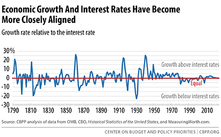
Growth has exceeded interest rates on average over the last two centuries, and has done so by greater margins in recent decades. From 1792 through 2025 — with our time period extending 10 years into the future for reasons explained in footnote 3 — annual growth has exceeded interest rates by an average of 0.9 percent.[3]
To be sure, that average is driven significantly by the periods of major wars, in which economic growth has exceeded interest rates by very large margins. In 1942, for example, nominal gross domestic product (GDP) grew 27 percent while the nominal interest rate was 2 percent, yielding a difference of 25 percent. During the War of 1812, the Civil War, and the two World Wars, economic growth has exceeded interest rates by an average of 12.4 percent; in general, the large increases in government spending that major wars require lead to rapid, though temporary, increases in economic growth.
The Great Depression, which sent the economy plummeting, significantly affected the relationship between economic growth and interest rates in the other direction. From 1930 through 1933, when the economy shrank but interest rates couldn’t fall below zero, interest rates greatly exceeded economic growth — by almost 23 percent, for example, in 1932. The very rapid economic recovery under the New Deal reversed the relationship once more, with economic growth exceeding interest rates (by an average of 6.5 percent from 1934 through 1938), much as during major wars.
Nevertheless, if we exclude war years and the abnormal Great Depression era, economic growth still exceeds interest rates on average over the nation’s history, though by a less striking 0.2 percent.[4] (See Table 1 and Figure 1.)
| TABLE 1 | |||
|---|---|---|---|
| How often has the economic growth rate exceeded interest rates, and by how much? | |||
| How often | By how much (percentage points) |
||
| Average | Median | ||
| All years, 1792-2025 | 57% | 0.9 | 1.0 |
| Major Wars and Great Depression era | 65% | 5.1 | 6.0 |
| 1792-2025, except major wars and Great Depression | 56% | 0.2 | 0.7 |
| 1947-2025 | 65% | 1.3 | 1.3 |
| 1947-1980 | 85% | 3.6 | 3.4 |
More specifically, even if we don’t count major wars or the Great Depression, economic growth has exceeded interest rates in 56 percent of the years from 1792 through 2025. Moreover, economic growth has exceeded interest rates by a greater degree since the end of World War II. Between 1947 and 2025, economic growth exceeds interest rates in almost two of every three years and, over that full period, by an average of 1.3 percent. In short, across our history, economic growth has exceeded interest rates more often than the reverse.
The relationship between economic growth and interest rates has become less volatile. That relationship can swing over a broad range in a very short time. This volatility, which primarily reflects volatile nominal GDP growth rates,[5] is declining (see Figure 1) because boom-and-bust economic cycles have become much less frequent and extreme. Even excluding major wars and the Great Depression era, the period from 1792 through the end of World War II includes 17 years in which either growth exceeded interest rates by more than 8 percent or interest rates exceeded growth by more than 8 percent. Since then, interest rates have never exceeded growth by more than 8 percent and economic growth has exceeded interest rates by that amount only once (by 15 percent in 1951).
Long-Run Debt Projections Are Very Sensitive to the Relationship Between Economic Growth and Interest Rates
Fiscal Sustainability and the relationship between economic growth and interest rates. The ratio of debt to GDP is a common and meaningful measure of fiscal sustainability.[6] When the nominal GDP growth rate exceeds the nominal interest rate, the government can run modest primary deficits and still have a stable or falling debt ratio. By contrast, when interest rates exceed economic growth, the government must run primary surpluses (i.e., revenues must exceed program costs) in order to stabilize or reduce the debt ratio. When economic growth rates and interest rates are the same, a primary balance will stabilize the debt ratio and primary surpluses will reduce it. (See Appendix 3 for the algebra behind these results.)
A simple, hypothetical example shows how important the relationship between growth and interest rates is for the long-run direction of the debt ratio. Imagine a country whose budget is in primary balance. Also assume that, in 2014, that country’s debt is 50 percent of its GDP. Finally, assume that in every year for 50 years, the country’s economy grows at a nominal 5 percent rate.
Figure 2 illustrates the stark effect of different economic growth and interest rate relationships for that hypothetical country. If economic growth equals interest rates in all years, then the country’s debt-to-GDP debt ratio will remain at 50 percent in all years. That, in essence, is fiscal sustainability because the debt ratio isn’t rising. But if interest rates exceed economic growth by 1 percentage point in all years, the debt ratio will grow to 80 percent after 50 years. If economic growth exceeds interest rates by 1 percent, the debt ratio will shrink to 31 percent of GDP after 50 years.
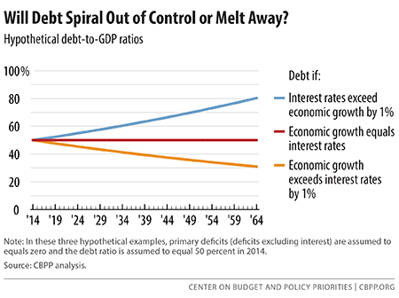
The growing debt caused by interest rates that exceed economic growth — and illustrated by the top line in Figure 2 — is sometimes called a “debt spiral.” Individuals who face extremely high interest rates on, say, credit card debt or “payday loans” have good reason to worry about their own debt spirals, since the rapid compounding of interest and debt can drive them into bankruptcy. But we shouldn’t generalize too much from the real problems that deeply indebted individuals face; the situation that the U.S. Treasury faces is much better because the interest rates it pays are always much lower than that of individuals. In fact, as we have shown, those interest rates are more often lower, rather than higher, than economic growth. And when that occurs and the budget is in primary balance, the burden of debt slowly melts away on its own, as the bottom line on Figure 2 shows.[7]
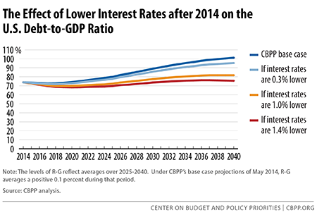
Alternative projections. Figure 3 shows the Center’s May 2014 “base case” projections of the debt ratio and what would happen if projected interest rates are lower than we assume.[8] Through 2024, those projections use CBO’s economic assumptions of spring 2014 (with projected growth exceeding projected interest rates through most of the coming decade). Thereafter and through 2040, projected interest rates exceed projected economic growth by an average of 0.1 percent, since they are based on CBO’s most recent long-term projections.
Figure 3 also shows what would happen if we reduced our assumed interest rates. Suppose we reduced our assumed rates by 0.3 percentage points starting in 2015. In that case, projected growth would exceed projected interest rates by an average of 0.2 percent after 2024 (rather than interest rates exceeding economic growth by 0.1 percent), in line with the non-war average across two centuries of U.S. history. As a result, the debt ratio would reach 95 percent by 2040, not 101 percent. Going further, if we reduced assumed interest rates by 1.4 percentage points starting in 2015 — so that, in line with the post-World War II average, projected growth exceeds projected interest rates by 1.3 percent — the debt ratio would equal 76 percent in 2040 and be heading downward.
Long-run projections, the “fiscal gap,” and the relationship between economic growth and interest rates. The fiscal gap offers a convenient way to summarize the long-run budget outlook in a single number. The fiscal gap is the average amount of program reductions or revenue increases that the government needs to implement over some future period to ensure that the debt is the same percent of GDP at the end of the period as it is today. Thus, the fiscal gap measures fiscal sustainability.
Under our May 2014 long-run budget projections, the fiscal gap through 2040 equals 1.0 percent of GDP. This means that stabilizing the nation’s finances through 2040 would require some combination of program cuts and tax increases totaling more than $180 billion per year if they went into effect in 2015 and grew with GDP.[9]
| TABLE 2 | ||
|---|---|---|
| If Interest Rates Are Lower, the Fiscal Gap Shrinks | ||
| Fiscal Gap through 2040 | Debt ratio in 2040 | |
| Percent of GDP | ||
| With interest rates assumed by CBPP (base case) | 1.0% | 101% |
| If rates are 0.3 percentage points lower starting 2015 | 0.8% | 95% |
| If rates are 1.0 percentage points lower starting 2015 | 0.3% | 82% |
| If rates are 1.4 percentage points lower starting 2015 | 0.1% | 76% |
But, as Table 2 shows, if interest rates are 0.3 percentage points lower than we assume, so that economic growth exceeds interest rates by an average of 0.2 percent after 2024, the fiscal gap through 2040 falls by one fifth; if economic growth exceeds interest rates by an average of 1.3 percent, the fiscal gap almost disappears.
In short, if the future relationship between economic growth and interest rates more closely aligns with the historical relationship, the long-term budget outlook may be somewhat less challenging than we, CBO, and some others assume.
Appendix 1:
The Data for 1792 through 2025
The data on the historical levels of the interest rate-growth differential (the IRGD, i.e., the R-G) build on nominal GDP growth data and nominal interest rate data.
GDP. The source of the data on nominal GDP growth from 1792 through 1930 is Louis Johnston and Samuel H. Williamson, What Was the U.S. GDP Then?, which covers calendar years 1790-2013.[10] For 1931 through 1939, we use the newly revised GDP data from the Bureau of Economic Analysis, which cover calendar years from 1929 on and calendar quarters from 1948 on. For 1940 through 2014, we use the GDP figures in OMB’s historical tables. For 2015 through 2025, we use CBO’s January 2015 estimates and projections of GDP growth. Because our interest rate data are necessarily calculated over fiscal years, we need to calculate GDP growth during fiscal years as well.
- Through 1842, the fiscal year was the calendar year, so we can use the Johnston-Williamson GDP figures directly.
- For 1843 through 1930, we obtain GDP figures for the fiscal year by averaging the Johnston-Williamson GDP for that calendar year and the preceding one; this approximates GDP over the period from July 1 through June 30, the fiscal year during that period. This also means that the growth of GDP from fiscal 1842 to 1843 (actually, it shrank) covers a six-month period, so we calculate the growth rate by squaring the ratio GDP1843/GDP1842.
- For 1931 through 1939, we obtain GDP figures for the fiscal year by averaging the BEA GDP for that calendar year and the preceding one, as above.
- For 1940 on, OMB and CBO show fiscal year GDP figures directly and take account of the change in the fiscal year that began in 1977.
Interest payments on debt held by the public. As described below, we calculate the interest rate on outstanding Treasury debt held by the public by dividing interest payments by debt. Of course, the concepts used for the numerator and denominator must be consistent for this calculation to be meaningful. (In general, the interest figures discussed here and the debt figures discussed in the next part of this appendix are those for the applicable fiscal years, so we don’t need to convert interest and debt data from a calendar-year basis to a fiscal-year basis.)
Unfortunately, data on payments of interest on debt held by the public are not readily available. Specifically, the budget functional category called “Net Interest” is complex. Within that function, subfunction 901 shows gross interest payments, including payments to U.S. government trust, special, and revolving funds, and so constitutes a figure far greater than just the interest payments to the public. The interest payments to other government funds are offset elsewhere: subfunction 902 shows the interest receipts of on-budget government trust funds; subfunction 903 shows the interest receipts of the Social Security trust funds; and subfunction 908 includes interest receipts that offset Treasury payments to revolving and special funds. But subfunction 908 also contains interest transactions between the Treasury and credit “financing accounts,” and other interest payments or receipts made directly between the public and agencies other than the Treasury. In addition, subfunction 909 portrays other investment-type net earnings of government agencies. There is no combination of subfunctions that represents interest payments on debt held by the public.
Fortunately, from 2004 on, OMB’s public budget database[11] shows a figure for interest payments on debt held by the public as a separate budget account within subfunction 901. Estimates are also shown going forward, consistent with presidential budget policies. And CBO likewise shows estimates going forward, consistent with its baseline. From 2004 on, we use these data in our calculations.
Of note, from 2004 on, the figure for interest payments on debt held by the public averages 95 percent of the combined levels of subfunctions 901 through 903, with only a very small amount of variation from year to year and no trend over time. The sum of those subfunctions represents gross Treasury debt payments minus the intragovernmental payments to trust funds and so approximates net interest payments on debt held by the public. But this persistent 95 percent figure strongly suggests that, for years before 2004, taking 95 percent of the net of subfunctions 901-903 would produce a much better approximation than simply using the sum of those three subfunctions. For lack of a better alternative, we do precisely that. Because subtotals for the three subfunctions exist from 1962 on, we are able to make what we believe are very good approximations of interest paid to the public for 1962 through 2003.
Before 1962, data on Treasury interest payments by subfunction are not available. Here, our ability to approximate payment of interest to the public is less certain. Nevertheless, we make what seems to be a reasonable approximation: we note that payments of interest on debt held by the public from 1962 through 2014 average 104 percent of the entire Net Interest function, although this figure varies from year to year. Nevertheless, it allows us to approximate interest payments to the public from 1940 through 1961, because OMB publishes totals for the Net Interest function back to 1940.[12]
Before 1940, we have little choice but to take the interest totals published by the Bureau of the Census in Historical Statistics of the United States.[13] Fortunately, before 1940, trust, special, and revolving funds were rare and small and the government did not engage in many other types of lending or borrowing transactions, beyond the longstanding approach of borrowing to finance deficits. As a result, the differences between gross and net interest payments are increasingly insignificant as one looks back further in time.
Interest rates. Because we are analyzing the effect of R-G values on the government’s debt, we must use the average effective interest rate on outstanding government debt rather than a broader measure of society-wide interest rates.[14] We calculate the government’s interest rate directly by dividing the (net) interest paid to the public — discussed above — over the course of the fiscal year by the average government debt held by the public during that fiscal year.[15] Because that interest rate constitutes a simple interest rate, we then convert it to a compound interest rate for the fiscal year (see Part 4 of Appendix 3). When discussing R-G, the R in question is this compound interest rate.
- End-of-fiscal-year debt from 1791 through 1939 is available from The Historical Statistics of the United States: Colonial Times to 1970.[16] Through 1842, the fiscal year coincided with the calendar year. In 1843, the start of the fiscal year was advanced to July 1. As a result, the interest for 1843 shown in Historical Statistics covered the six months from January through June. We doubled that amount of interest before dividing it by the average level of debt during those six months, thereby producing an annualized interest rate.
- End-of-fiscal-year debt from 1940 through 2014 is available from the U.S. Budget, Historical Tables.[17] This allows us to calculate interest rates for 1941 through 2014. Beginning with fiscal year 1977, the start of the fiscal year was pushed back one quarter, to October 1. Therefore, the calculation of average debt over fiscal year 1977 requires a figure for debt as of September 30, 1976. This figure is available in the Historical Tables, which show data not only for fiscal years but also for the “transition quarter” of July 1, 1976, through September 30, 1976.
- To calculate the interest rate for 1940, we need the average debt during that year and so need comparable debt figures for 1939 and 1940 as well as a comparable interest figure for fiscal year 1939. But the debt and the interest series for 1791 through 1939 (the first bullet above) are not strictly comparable to the series from 1940 through 2014 (the second bullet above). Fortunately, the necessary debt and interest data are available in other series in the Historical Statistics.[18]
- For 2015 through 2025, we calculate interest rates from interest and debt figures in CBO’s January 2015 database.
Two calculations of average R-G. We use two different versions of the R-G time series in our analysis. The first includes data for all years from 1792 through 2025 except for the 1835-1838 period. We exclude that four-year period because the U.S. government had paid off its entire debt in 1835-1836. The implicit interest rate, which is calculated by dividing interest payments to the public by debt held by the public, thus cannot be calculated for this period.
The second version, which we emphasize in this analysis, excludes the data from the Great Depression era as well as from years in which the United States was involved in major wars. In addition, data from the year preceding the declaration of war and following the conclusion of the war have been omitted because those data likewise tend to be idiosyncratic. This version, then, excludes the following years: 1811-1816 (War of 1812), 1835-1838 (no debt), 1860-1866 (Civil War), 1916-1919 (U.S. involvement in World War I), 1929-1938 (Great Depression era), and 1940-1946 (World War II). The rationale for excluding the war years from the data is that participation in wars tends to lead to increases in nominal economic growth rates, which in turn implies very negative R-G values. These values skew the overall observed values of R-Gs downward, which is why excluding war years increases the average R-G. As noted in Table 1, in the excluded years the R-G averaged negative 5.1 percent.
Appendix 2:
Why Long-Run Projections Need Not Be Dynamic
A perpetually rising debt-to-GDP ratio is unsustainable and therefore unrealistic as a forecast of what will actually happen. At some point policymakers will decide to take action or be forced by events to take action to achieve fiscal sustainability. And as Paul Krugman and others have pointed out,[19] a high debt ratio does not necessarily translate into higher interest rates for countries, like the U.S., the U.K., and Japan, that can borrow in their own currencies over a broad range of debt-to-GDP ratios well beyond current U.S. levels. For these reasons, long-run forecasters such as GAO, OMB, CBO, Gale-Auerbach, and others generally do not try to introduce dynamic feedback effects of rising debt on interest rates and growth into their forecasts.
Long-run debt projections provide a measure of the long-run debt problem at a particular moment of time: the amount of primary deficit reduction (revenue increases and program cuts, not including the associated interest savings) needed to restore fiscal sustainability. Because a solution to the debt problem means, at a minimum, achieving a constant debt ratio, it is sufficient when measuring the size of the long-run problem to use interest rates and growth rates consistent with a constant debt ratio, rather than with an exploding one.
Suppose, for instance, that long-run projections were created in two steps. In Step 1, program spending, revenues, and interest are projected consistent with assumed Rs and Gs that ignore the bad consequences of exploding debt. For example, Step 1 might show the debt ratio rising from 75 percent to 125 percent over 40 years. In Step 2, assumed Rs are increased and Gs are decreased to reflect the possible unfortunate dynamic consequences of this exploding debt, such as higher interest rates and slower economic growth. This would make the picture still worse; instead of rising to 125 percent, the debt ratio might rise to (say) 140 percent.
But now imagine that Congress enacts enough deficit reduction to solve the problem revealed by Step 1, that is, to stop the debt ratio from rising from 75 percent to 125 percent and instead stabilize it at 75 percent (assuming normal Rs and Gs). With debt stabilized at 75 percent, the increased Rs and decreased Gs calculated in Step 2 will not occur. In short, solving the problem revealed by Step 1 is fully sufficient to solve the additional possible problem revealed by Step 2. Therefore, the calculations in Step 2 are not needed to describe the size of the problem — that is, to inform Congress about how much combined program cuts and revenue increases are needed to stabilize the debt.
Meanwhile, the calculations in Step 2 would be highly uncertain because the United States has no experience of multi-decade periods of debt ratios exceeding 100 percent of GDP and growing indefinitely — although Japan’s ability to borrow at low interest rates with a very high debt-to-GDP ratio suggests the U.S. is far from a danger point. Instead of making dynamic estimates that would be highly uncertain, inevitably controversial, subject to misuse and misinterpretation, and unnecessary in informing policymakers how much deficit reduction is needed to stabilize the debt ratio, those who make long-run projections generally — and wisely — skip Step 2 entirely.
Appendix 3:
The Algebra of R, G, and Long-Run Budget Projections
This appendix contains six parts. In the first, we show how debt evolves from year to year as a function of prior debt, primary deficits, interest rates, and GDP growth rates. Assuming constant interest rates, GDP growth rates, and primary deficits (as a percent of GDP), we derive an equation for debt in any year as a function of the starting debt and those variables.
In the second part, we use the equations from the first part to derive the conditions under which the debt ratio rises or falls; significantly, this is a function of, among other conditions, R-G, which is the central topic of this analysis.
In the third part, we show that when R-G = 0, the evolution of the debt ratio over time can be expressed very simply, which facilitates an intuitive understanding of the more complex equations derived in the second part.
In the fourth part, we examine whether the value of R-G or the level of the primary deficit is more important in determining whether the debt ratio is stable. We find that the answer depends upon the initial debt ratio we seek to stabilize. At the current level of the debt ratio, however, R-G is the more important factor.
In the fifth part, we explain why the interest rate that we use in the first four parts and discuss in our analysis is a compound rate (over the course of a year), not a simple interest rate. We derive a simplified equation for the compound rate as a function of the simple rate.
In the sixth part, we contrast our equation for the evolution of debt from one year to the next with the two equations commonly used in the academic literature on debt. We demonstrate that these two alternatives are slightly less accurate simplifications.
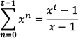
Part 1: The evolution of debt as a function of R, G, and the primary deficit p. In our terminology, which is relatively standard, debt and GDP in year t are denoted as Dt and Yt, respectively.[20] Debt and GDP in the starting year, t=0, are thus D0 and Y0. GDP in any year equals the GDP in the prior year times [1 plus the nominal GDP growth rate g], written as:
As a result, if g is constant, GDP in year t can be written as:
Finally, the nominal compound interest rate is r, and as with G, we designated R as: [21]
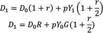
To derive a general equation for the evolution of debt over time, we start by expressing debt in year one as a function of debt in year zero and other variables. Specifically, the debt at the end of year one equals the debt at the end of year zero plus the primary deficit p (shown as a percent of GDP in year 1) plus the interest cost of the debt and of half of the primary deficit.[22]
Rearranging the terms, the debt at the end of year one is the sum of the existing debt, interest on the existing debt, the new debt (i.e., the primary deficit), and interest on the new debt. In calculating interest on the primary deficit, we note that the primary deficit does not spring into being, fully formed, on the first day of the fiscal year. Rather, the total primary deficit accumulates over the course of the fiscal year; for that reason, the average level of the primary deficit during the year — which is what we pay interest on — can be well approximated as one-half the total primary deficit for the year. The debt at the end of the fiscal year can thus be written as:
Factoring out D0 and pY1 where applicable and noting that Y1 = Y0G yields
To simplify the process of deriving equations, we use C to represent
For the purpose of this appendix, we assume that R, G, and p are constant in all years. Therefore, for year 2, we have:
Substituting the amount of debt at the end of year 1 (that is, D1) into this equation yields
Rearranging,
A pattern begins to emerge, but one more iteration will make it clear. In year three, we start with:
Substituting for D2, we see
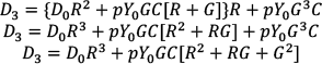
At the end of every year t, the debt is equal to the initial debt times Rt for each year plus the primary deficit in year 1 (that is, pY0G), with this term growing both as a function of the compound interest rate and the size of the economy.
The term in brackets is a summation of the following pattern:
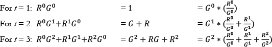
Skipping the intermediate step, here’s the bracketed term for t = 4:
Most generally, the bracketed term can be summarized as follows for all years t > 1:
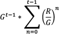
Therefore, in any year t > 1, the debt level equals:
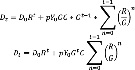
The power series tells us that
Let
Part 2: Stabilizing the debt ratio. Now let’s express the debt as a percent of GDP by dividing all the terms by Yt or by its equivalent, Y0Gt.
Finally, let’s designate the initial debt-to-GDP ratio
From this, we can determine what conditions keep the debt ratio stable, that is, we can find the parameters that ensure
If we impose the condition that the debt ratio must be constant, we have:
The relationship between r, g, p, and the initial debt ratio A can be summarized as follows. If p is equal to 0, that is, if there is no primary deficit, then B must equal 1 to maintain the debt ratio. And if B = 1, then r = g (recall that
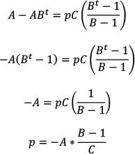
Recall again that
So for the debt ratio to be constant over time (at level A):
- if p (the primary deficit) equals 0, then R-G must also equal 0, and vice versa;
- if p is positive (so we are running primary deficits), then R-G must be negative, i.e., the interest rate must be lower than the economic growth rate in order to offset the primary deficits; and
- if p is negative (so that we are running primary surpluses), then R-G is positive. In other words, if interest rates exceed the economic growth rate, primary surpluses would be needed in order to offset that fact and keep the debt ratio stable.
Part 3: When R equals G, simplified. When R equals G, equation 1.2 above becomes far simpler, since many terms drop out. To start, the term generally represented as
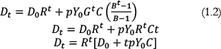
To express debt as a percent of GDP, we now divide both sides of the equation by Yt. But since Yt = Y0Gt = Y0Rt, we can divide the left side of the equation by Yt and the right by Y0Rt, yielding:
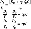
This final equation is an especially simple way of seeing that, to keep the debt ratio constant at its initial level when R equals G, the primary deficit must be zero.
Part 4: Which is more significant in stabilizing the debt — r-g or the primary deficit? Perhaps this question is metaphysical. But one analytical approach is to normalize the range of r-g values and the range of primary deficits and then compare how changes in each of these factors over its normalized range affect the debt ratio.
The standard deviation of r-g from 1947 through 2014 is 3.5 percentage points and the standard deviation of primary deficits over the same period is 2.5 percent of GDP; we take these to be the normal ranges of these factors. Using equation 2.2, we find that when the initial debt ratio “A” is 50 percent of GDP, a positive r-g value of one standard deviation would require the government to run offsetting primary surpluses of just about one standard deviation to keep the debt ratio stable. Likewise, if r-g were negative by one standard deviation, debt would remain stable even if the government ran primary deficits of one standard deviation. So if the initial debt ratio is 50 percent of GDP, r-g and primary deficits can be thought of as equally important in stabilizing debt.
If the initial debt ratio were only 25 percent of GDP, however, the government could offset the effect of a positive r-g value of one standard deviation by running a primary surplus of about one-half of a standard deviation. In this case, then, primary deficits are about twice as significant as r-g in stabilizing debt. On the other hand, if the initial debt ratio were 75 percent of GDP (slightly above its current level), the value of r-g is about 40 percent more important than the size of the primary deficit in stabilizing the debt ratio. In short, the higher the initial debt ratio, the more significant is r-g relative to the primary deficit. This result should be intuitive.
Part 5: “r” represents compound, not simple, interest. In part 1, our initial equation 1.1 includes a term representing interest; we multiply the existing debt and one-half the primary deficit by the interest rate r. Of note, r is a compound interest rate because at the margin the Treasury borrows to pay interest, and so pays interest on the interest.
To illustrate, consider a nation with primary balance and a starting debt of $100 billion, and imagine that its treasury borrows throughout the year by issuing securities with a simple interest rate s of 4.0 percent. For simplicity, let’s say it pays interest twice a year at one-half the interest rate s. The interest cost in the middle of the year is
And this $2 billion of interest itself incurs an extra borrowing cost to the tune of
Which, again, incurs an extra borrowing cost equaling
Interest costs for one-half the year will be the sum of the terms above, plus the additional terms from the continuation of this series. Using D to designate the starting debt for the year (in this example, $100 billion), i/2 to designate interest cost during half the year, and s to designate the simple interest rate (in this case, 4 percent), the sum of the series (when continued) is
The limit of a power series that starts at n = 0, rather than n = 1, has a known answer, so below we start the series at n = 0 and then subtract the term where n = 0; because
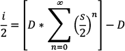
Because s < 1, this series converges, and using the formula for its limit, we see
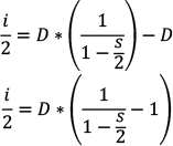
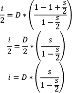
So for a simple interest rate s, the compound interest rate r that applies to the starting debt is:
By the same reasoning, the same r applies to primary deficits as they accumulate over the year, that is, to
In Appendix 1, we noted that we obtained interest rates by dividing interest paid during the year by the average amount of debt outstanding during the year. However, that quotient produces a simple rather than a compound interest rate. We therefore used those quotients and equation 5.1 above to derive the compound interest rate r that we display and discuss in the body of this analysis; along with g and p, it is that compound rate r that is one of the key variables in determining the evolution of debt.
Part 6: The academic literature uses less accurate but simpler equations. When the academic literature discusses the evolution of debt from year to year, it generally portrays an equation showing the change in debt as a percent of GDP from year zero to year 1. That is, it expresses D1/Y1 - D0/Y0 as a function of r, g, the initial debt ratio D0/Y0, and the primary deficit p. In this part we derive such an equation for D1/Y1 - D0/Y0 consistent with Part 1. We then contrast our result with those commonly found in the academic literature.
Recall that Part 1 of this appendix starts, in equation 1.1, by showing how debt in year 1 relates to debt in year zero, given r, g, p, and Y.
From here, we can display the debt ratio
As in Part 1, we substitute C for
We next divide all terms by Y1 and subtract
We next substitute Y0G for Y1 on the right-hand side and factor out
Finally, note that
About half of the academic literature shows precisely this equation (perhaps with different terminology) in every respect except one: the term C is omitted, thus:[23]
Working backwards from this equation, the starting equation, corresponding to our equation 1.1, must be:
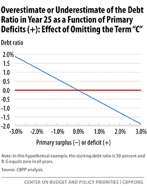
Evidently, then, this starting equation 6.3 includes the cost of new debt - the primary deficit - but not any interest on it. This is equivalent to assuming that the primary deficit is incurred entirely on the last day of the fiscal year. As a result, this simpler equation will underestimate the significance of primary surpluses or deficits on the evolution of debt over time. If the nation is running primary deficits, this equation will underestimate future debt; if the nation is running primary surpluses, the equation will overestimate future debt.
Figure 4, below, shows that this simplification has only a small effect. Specifically, it shows that if the debt ratio starts at 50 percent and r = g, then after 25 years of primary deficits of 3 percent of GDP, the debt ratio would be underestimated (relative to our equation 2.1) by less than 2 percent of GDP. Similarly, after 25 years of primary surpluses of 3 percent of GDP, the debt ratio would be overestimated by less than 2 percent of GDP.
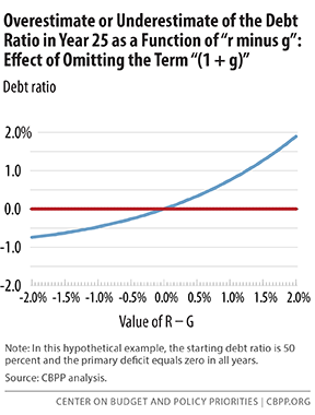
It should also be noted that, if one accepts the simplification that primary deficits occur only on the last day of the fiscal year, the analogous subsequent equations in Part 1 (such as the equation for Dt,
The other half of the academic community uses an equation for the year-to-year increase in the debt ratio that is simpler still; not only does it omit the term C, it also omits the term (1+g). It thus reads
It is not clear what initial assumptions would lead to this simplified equation. Be that as it may, because it does not divide existing debt by (1+g), this equation overestimates the significance of r-g.
If r-g is negative, equation 6.4 overestimates the speed at which existing debt melts away; if positive, it overestimates the speed at which existing debt spirals. Again, this simplification has only a small effect. Figure 5 shows that if the debt ratio starts at 50 percent and primary deficits equal zero, then after 25 years of r-g of negative 2 percent, the debt ratio would be underestimated (relative to our equation 6.1) by three-quarters of a percentage point. After 25 years of r-g of positive 2 percent, the debt ratio would be overestimated by less than 2 percentage points.
And like equation 6.2, used by the other half of the academic community, equation 6.4 also understates the significance of primary deficits by omitting the term C.
End Notes
[1] The text, tables, and figures in this analysis show the effect on debt when G is greater than R — i.e., when G-R is positive. However, the algebra behind the relationships, as explained in Appendix 3, is more comprehensible when it is framed in terms of R-G rather than G-R. Therefore, in the body of the analysis, we discuss what happens when G-R is positive, whereas in the three technical appendices and in the spreadsheet available on our website (at ), we discuss what happens when R-G is negative. R-G is frequently called the Interest Rate-Growth Differential, or the IRGD. The precise meaning of R-G can be confusing, however. For instance, in Capital In the Twenty-First Century, Thomas Piketty maintains that R-G will become increasingly positive over time and exacerbate the inequality of income and wealth. But he is discussing a very different R — the average return on private-sector capital investment. The R that we consider in this analysis refers to the average interest rate that the U.S. Treasury pays on debt held by the public. While these two different Rs are somewhat related, there is every reason to expect Treasury interest rates to be substantially lower than private-sector rates of return.
[2] Richard Kogan, Kathy Ruffing, Paul N. Van de Water, and William Chen, “CBPP’s Updated Projections Show Long-Term Budget Outlook Is Significantly Improved but Remains Challenging.” Center on Budget and Policy Priorities, May 5, 2014, https://www.cbpp.org/cms/index.cfm?fa=view&id=4139.
[3] Our two-century averages include CBO’s implicit assumption about economic growth and interest rates from 2015 through 2025, derived from its January 2015 baseline, because those figures are consistent with specific CBO projections of the U.S. budget under the circumstances that now exist, and because we are attempting to evaluate the assumption that positive interest rates will exceed economic growth rates for the indefinite future, starting after 2025. However, the two-century averages we calculated would have been virtually identical if we had used data through 2014 rather than through 2025. We explain the data, its sources, and our calculations in Appendix 1.
[4] When excluding war years and the Great Depression era from our calculations, we also exclude the year immediately before and immediately after in each case, since they, too, often show abnormal results.
[5] This is apparent from the data in the linked spreadsheet but cannot be quantified directly because, as we explain in footnote 14 (Appendix 1), the interest data for any particular year is a rolling average of interest rates on all outstanding debt, not just on newly issued securities, and so is already smoothed to some extent.
[6] Sustainability is conventionally defined as a ratio of debt to GDP that remains roughly constant over time. If the debt ratio rose without limit, then interest costs would likewise rise without limit, eventually consuming the entire economy. Of course this could not happen, but the harm to the nation would become excessive well before interest costs reached 100 percent of GDP. For perspective, note that interest costs are currently 1.3 percent of GDP, above the two-century average of about 1 percent but less than half the historical high points, which occurred in 1985 and 1995. This figure is projected to rise because budget projections continue to show primary deficits and because the Federal Reserve is expected to raise interest rates as the economic recovery progresses. (The standard explanation of the economic harm caused by an excessive or constantly rising debt ratio is that it would crowd out productive private-sector investment, though not when the economy was operating well below capacity.)
[7] Besides paying lower interest rates, the government has additional advantages over indebted individuals or businesses. For example, it can raise revenues, whereas individuals generally cannot choose to increase their wages or businesses to increase their profits. In addition, the Federal Reserve holds some of the Treasury’s debt securities. This fact keeps some debt out of the hands of creditors, and the Fed returns its interest earnings to the Treasury; indebted individuals and businesses have no comparable advantages.
[8] Kogan et al.
[9] Technically, eliminating a 1.0 percent fiscal gap requires primary (non-interest) deficit reduction equal to 1.0 of GDP on a present-value basis. For simplicity, we describe this as program cuts and tax increases of 1.0 percent of GDP in each year over the 2015-2040 period. But one could, and almost certainly should, cut primary deficits by substantially less than 1.0 percent of GDP in the short term, given that the economy has not yet fully recovered from the Great Recession. If deficit reduction is smaller than 1.0 percent of GDP up front, it needs to be bigger than 1.0 percent of GDP later in order to reduce the 2015-2040 fiscal gap to zero.
[10] Available at http://www.measuringworth.com/usgdp/. Used by permission.
[11] The public budget database is found at http://www.whitehouse.gov/omb/budget/Supplemental/.
[12] Available at http://www.whitehouse.gov/omb/budget/Historicals/. Debt is shown in Table 7.1. The totals for the Net Interest function from 1940 appear in Table 3.1; subtotals by subfunction from 1962 appear in Table 3.2.
[13] Available at http://www2.census.gov/prod2/statcomp/documents/CT1970p2-01.pdf. Interest is shown in Series Y 461 of that document.
[14] Ideally, we would want to know the average effective interest rate on newly issued Treasury debt in a given year. But that information is not available for the more distant past. Therefore, we use the implicit interest rate on outstanding Treasury debt, derived as the ratio of Treasury interest payments to the public to Treasury debt held by the public. This interest rate on outstanding debt, though volatile, is nonetheless smoother than the rate on newly issued debt. In that respect, the interest rates for any given year shown in the spreadsheet available on our website (at ) are already smoothed to some extent. Although this smoothing, though necessary, makes our calculations less than useful for an economic historian trying to examine, for example, interest rates on newly issued Treasury debt during the 1887-1888 recession, this smoothing makes no difference to our examination of long-term historical averages and trends.
[15] Public commentary on Treasury interest rates often focuses on the rate paid by the Treasury on its flagship 10-year bonds. But that figure overstates Treasury interest rates because the mix of Treasury securities always has an average maturity that is shorter than 10 years — generally shorter than five years.
[16] Available at http://www2.census.gov/prod2/statcomp/documents/CT1970p2-01.pdf. Debt is shown in Series Y 338 of that document. (Debt is also shown in other series in that document, but the debt figures in Series 493 are in error from 1791 through 1842; that series shows start-of-year debt rather than end-of-year debt for those years and is therefore missing one year when it correctly starts portraying end-of-year debt in 1843.)
[17] Available at http://www.whitehouse.gov/omb/budget/Historicals/. Debt is shown in Table 7.1.
[18] Historical Statistics, Series Y 490 and Y 485, respectively.
[19] http://krugman.blogs.nytimes.com/2013/02/24/debt-spreads-and-mysterious-omissions/
[20] By longstanding convention, budget documents show GDP as the average over a fiscal year but show debt at the end of that fiscal year. As a result, debt/GDP ratios as commonly displayed are almost always overstated very slightly. However, this convention makes no difference to the algebra associated with calculating the evolution over time of the debt/GDP ratio.
[21] To make this paper easier to read, we use an upper case “G” in the body of this paper when referring to the GDP growth rate, although it is shown in this appendix as “g.” Likewise, in the body of the paper we use an upper case “R” to refer to the interest rate shown here as “r”. If you prefer consistency between the body of the paper and this appendix, please note that R-G = (1+r) - (1+g) = r-g, so that the two subtractions are identical.
[22] The primary deficit is the deficit excluding interest costs, i.e. the amount by which program costs exceed revenues. Since we show debt as a positive figure, we also show primary deficits p*Y as positive figures so that deficits add to debt. A primary surplus would be -p*Y. For the purpose of this paper, what we call the primary deficit is synonymous with a cash deficit and is assumed to be financed entirely by additional borrowing. Federal budget accounting, while largely done on a cash basis, includes some exceptions. The most significant is that the cash the Treasury borrows to make direct loans (e.g., to students) is offset in budget accounting by the present value (to the government) of the acquired loan asset. The difference between the recorded deficit and the pure cash deficit is called “other means of financing.” Therefore, when we refer to deficits in this analysis, we mean deficits as recorded plus other means of financing; likewise, when we refer to primary deficits, we mean primary deficits as recorded plus other means of financing. An alternative and more intuitive approach would be to use the term deficits to mean deficits as recorded, and to use the term debt to mean debt net of financial assets. The equations in this appendix are equally valid under the standard and the alternative approaches to these terms.
[23] Some authors display a primary deficit as a negative amount and thus end the equation with -p rather than +p, but that is just terminology. We use the same sign for debt and deficits to reflect that deficits add to debt.
More from the Authors

Areas of Expertise