What Was Actually in Bowles-Simpson — And How Can We Compare it With Other Plans?
Many policymakers have said that they “support,” “endorse,” or otherwise look favorably on “Bowles-Simpson” — the budget plan that Erskine Bowles and Alan Simpson issued in December 2010 as co-chairs of President Obama’s National Commission on Fiscal Responsibility and Reform.[1] But despite this apparent widespread support, many policymakers and opinion leaders do not understand the specifics of what Bowles-Simpson actually included. For instance, a bipartisan budget plan offered in the House this spring claimed the Bowles-Simpson moniker. Yet that plan departed very substantially from Bowles-Simpson in key respects.[2]
In anticipation of a renewed focus on Bowles-Simpson in the months ahead, policymakers and opinion leaders in the budget debate need to have a solid grasp of what the plan actually proposed. This is particularly the case if Bowles-Simpson is held up as a budgetary benchmark for assessing other proposals. How much deficit reduction did Bowles-Simpson actually entail, how much would it raise revenues, and what ratio of revenue raisers to program cuts did it encompass? To make those assessments accurately, it is essential to understand three key issues.
The Treatment of Social Security
The Bowles-Simpson plan included revenue and benefit changes designed to restore long-term solvency to the Social Security trust fund. For purposes of presentation, the Bowles-Simpson documents and public statements by the co-chairmen excluded the Social Security solvency proposals in some aspects of their presentation and included those proposals in others. The Social Security proposals were usually not counted in the deficit reduction totals or in the ratios of spending cuts to revenue increases, as the co-chairs described the Social Security proposals as not having been done for the purpose of deficit reduction. These proposals were included in calculations of the resulting levels of revenues, spending, deficits, and debt. In this analysis, we present the plan using the same approach as the co-chairs.
Treatment of upper-income tax cuts. Second, when the Bowles-Simpson plan listed the savings that its proposed policies would achieve, it used a revenue baseline that assumed that the tax cuts President Bush and Congress enacted in 2001 and 2003 would expire for incomes over $250,000 for couples ($200,000 for singles). After Bowles and Simpson issued their plan (and starting with the budget negotiations of 2011), policymakers of both parties decided to measure revenue changes from a different, “current policy,” baseline — i.e., a baseline that assumes that policymakers would extend all of the Bush tax cuts and almost all other expiring tax provisions.[3] Budget organizations such as the Concord Coalition, the Committee for a Responsible Federal Budget, and the Center on Budget and Policy Priorities also now measure budget plans against a current policy baseline.
Compared with a current policy baseline, a policy that lets the upper-income and certain other tax cuts expire saves $1.1 trillion over the 2013-2022 period and produces about another $170 billion of interest savings. Bowles-Simpson included those savings, but rather than listing them as savings, it assumed that policy change as part of its baseline.
Enacted spending cuts. Finally, when Bowles and Simpson crafted their plan, the most recent year for which policymakers had enacted full-year appropriations was 2010, and the Congressional Budget Office (CBO) baseline for discretionary funding reflected the 2010 levels, adjusted for inflation in future years. Since then, policymakers have enacted large cuts in discretionary programs; indeed, they have enacted 70 percent of the discretionary savings that Bowles-Simpson called for. Under the caps on discretionary funding in last year’s Budget Control Act (BCA), discretionary spending will be $1.5 trillion lower over 2013-2022 than under CBO’s 2010 baseline. Including the associated interest savings, the total budget savings reach $1.7 trillion.
Summary of Updated Bowles-Simpson Estimates
To assess Bowles-Simpson today so that policymakers can compare it with other plans, one must look at the Bowles-Simpson savings over 2013-2022, relative to a current policy baseline. One must also account for the $1.5 trillion in discretionary spending cuts that policymakers have since enacted. When that is done, the results show that:
| Table 1 Summary of Original Bowles-Simpson Plan |
||
| Total plan | Not yet enacted | |
| Ten-year cumulative totals in trillions of dollars | ||
| Revenue increases | $2.6 | $2.6 |
| Program cuts | $2.9 | $1.4 |
| Interest savings | $0.8 | $0.6 |
| TOTAL deficit reduction | $6.3 | $4.6 |
| Ratio, program cuts to revenue increases | ||
| Not counting interest | 1.1 to 1.0 | 0.5 to 1.0 |
| Counting interest | 1.4 to 1.0 | 0.8 to 1.0 |
| Note: Covers 2013 through 2022; excludes Social Security solvency proposals; measured relative to current policy; may not add due to rounding. | ||
| Table 2 Deficit Reduction under the Original Bowles-Simpson Plan Extended to cover 2013-2022; dollars in billions |
|||||||||||
| 2013 | 2014 | 2015 | 2016 | 2017 | 2018 | 2019 | 2020 | 2021 | 2022 | 10-yr total | |
| Revenue increases: | |||||||||||
| Tax reform | 20 | 40 | 80 | 90 | 105 | 120 | 150 | 180 | 215 | 250 | 1,250 |
| Revenue increases built into baseline | 49 | 62 | 89 | 99 | 110 | 121 | 130 | 138 | 148 | 157 | 1,103 |
| Increase gas tax 15 cents | 2 | 7 | 11 | 16 | 18 | 18 | 18 | 18 | 18 | 18 | 144 |
| Chained CPIa: revenue effect | 2 | 3 | 5 | 7 | 8 | 10 | 11 | 12 | 14 | 16 | 88 |
| Subtotal | 73 | 112 | 185 | 212 | 241 | 269 | 309 | 348 | 395 | 441 | 2,585 |
| Mandatory health programs | 19 | 31 | 33 | 37 | 43 | 49 | 58 | 65 | 70 | 75 | 480 |
| Other mandatory programs/fees: | |||||||||||
| Chained CPIa | 1 | 2 | 3 | 4 | 5 | 6 | 7 | 8 | 9 | 10 | 55 |
| Other mandatory programs/fees | 10 | 13 | 18 | 22 | 25 | 29 | 32 | 36 | 38 | 40 | 263 |
| Subtotal | 11 | 15 | 21 | 26 | 30 | 35 | 39 | 44 | 47 | 50 | 318 |
| Appropriated (discretionary) programs: | |||||||||||
| Security | 61 | 86 | 101 | 117 | 133 | 148 | 163 | 178 | 193 | 208 | 1,386 |
| Non-Security | 27 | 36 | 48 | 57 | 65 | 73 | 81 | 90 | 98 | 107 | 682 |
| Subtotal | 88 | 122 | 148 | 174 | 197 | 221 | 244 | 267 | 291 | 316 | 2,068 |
| TOTAL deficit reduction policies: | |||||||||||
| Revenue increases | 73 | 112 | 185 | 212 | 241 | 269 | 309 | 348 | 395 | 441 | 2,585 |
| Program reductions | 118 | 168 | 203 | 237 | 270 | 305 | 341 | 376 | 408 | 441 | 2,866 |
| TOTAL | 191 | 280 | 388 | 448 | 511 | 574 | 650 | 725 | 803 | 882 | 5,450 |
| Resulting reductions in interest costs | 1 | 3 | 6 | 17 | 38 | 72 | 107 | 144 | 187 | 234 | 807 |
| Total: policies and interest savings | 191 | 283 | 394 | 466 | 549 | 645 | 756 | 869 | 989 | 1,116 | 6,257 |
| Addendum: Social Security solvency: | |||||||||||
| Increase the “taxable maximum” | 5 | 8 | 12 | 15 | 19 | 22 | 26 | 30 | 35 | 40 | 212 |
| Chained CPIa | 3 | 5 | 8 | 10 | 12 | 15 | 17 | 19 | 22 | 25 | 136 |
| Benefit improvements | 0 | 0 | 0 | 0 | 0 | -5 | -6 | -5 | -4 | -3 | -34 |
| Subtotal | 8 | 13 | 20 | 25 | 31 | 32 | 37 | 44 | 53 | 62 | 325 |
| Resulting reductions in interest costs |
0 | 0 | 0 | 1 | 2 | 4 | 6 | 8 | 11 | 14 | 45 |
| May not add due to rounding. Sources: Moment of Truth Project, Updated Estimates of the Fiscal Commissions Proposal, June 29, 2011; author’s extension for 2022; adjustments for current policy revenue baseline and CBO’s 2010 discretionary baseline based on data from CBO and the Joint Committee on Taxation. a) The “chained CPI” refers to a proposal to alter the way the Consumer Price Index is measured; a number of analysts believe the proposal would measure inflation more accurately, slightly reducing the measure. Because the tax code, Social Security, and some other federal programs such as Supplemental Security Income are indexed to the CPI, the proposal would cut spending and raise revenues. |
|||||||||||
- Over 2013-2022, Bowles-Simpson called for $6.3 trillion in deficit reduction — $5.5 trillion in policy savings and about $800 billion in interest savings. (That figure excludes Bowles-Simpson’s Social Security solvency proposals, consistent with their presentation of the plan’s deficit reduction totals; see the box on page 2.)
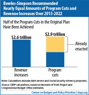
- The $5.5 trillion in policy savings in the Bowles-Simpson plan consists of almost $2.9 trillion in program cuts and almost $2.6 trillion in revenue increases — that is, 53 percent from budget cuts and 47 percent from revenue increases, or almost a 1-to-1 ratio of program cuts to revenue increases.
This nearly 1-to-1 ratio does not include the interest savings. If one counted interest savings as a spending reduction, the ratio is 59 percent in spending cuts to 41 percent in revenue increases, or a 1.4-to-1 ratio of program cuts to revenue increases.
Bowles-Simpson was typically described as having a 2-to-1 ratio, but that is because the co-chairs assumed the expiration of the upper-income tax cuts as part of their baseline and thus did not count the revenue savings in their ratio. They also estimated higher interest savings (which counted under their plan as a spending reduction) than our analysis does because the interest rates projected at that time were higher than interest rates now are projected to be. - Of the nearly $2.9 trillion of program cuts in the Bowles-Simpson plan, about half — or just under $1.5 trillion — have already been enacted. If one excludes the enacted savings:
- The Bowles-Simpson plan would achieve an additional $4.6 trillion in deficit reduction over ten years. (This doesn’t include the small savings in the first ten years from the plan’s Social Security proposals.)
- The majority of the remaining savings in the plan is on the revenue side: for every $0.54 of additional spending cuts, there would be $1.00 in new revenue under the Bowles-Simpson plan (or 35 percent budget cuts and 65 percent revenue increases), excluding interest savings.
- If one counts interest savings as a spending reduction, then the ratio of the remaining savings would be 43 percent program reductions and 57 percent revenue increases, or $0.76 of spending cuts for each $1.00 of revenue raisers.
The figures in this summary are shown in Table 1.
Setting a Deficit Reduction Target
Many policymakers and analysts agree that the minimum essential goal for a deficit reduction package is to “stabilize” the debt in the decade ahead — that is, to ensure that the debt stops growing faster than the economy (i.e., Gross Domestic Product, or GDP). Stabilizing the “debt-to-GDP” ratio is essential to prevent a debt explosion in coming decades, which would risk a financial crisis and weaken the economy over time. To achieve this goal over the 2013-2022 period relative to a current policy baseline would require roughly $2 trillion of deficit reduction (including interest savings) on top of the $1.7 trillion of savings already enacted.[4]
As explained above, the Bowles-Simpson plan over 2013-2022 would achieve $4.6 trillion of deficit reduction on top of the $1.7 trillion of already enacted savings, measured relative to a current policy baseline. This $4.6 trillion total is more than twice what is needed to stabilize the debt ratio and thus explains why the Bowles-Simpson plan goes well beyond stabilizing the debt as a share of the economy and in fact significantly reduces the debt-to-GDP ratio.
As policymakers consider various deficit reduction packages, they should keep in mind what various amounts of deficit reduction will achieve in terms of managing the national debt. They should also be aware of the mix and nature of program reductions and revenue increases used to achieve these goals. The challenge will be to strike the right balance.
The Dollar Targets in Bowles-Simpson
Here are the facts, summarized in three tables.
- Table 2 shows the dollar amount of tax increases and program cuts that Bowles-Simpson proposed relative to current policy over the ten-year “budget window” of 2013-2022 — $5.5 trillion (not counting the Social Security proposals). It shows that 53 percent of the savings came from program cuts and 47 percent from revenue increases, or $1.11 in program cuts for every $1.00 in revenue increases.
- Table 3 shows that policymakers have already achieved (or have locked in for future years) $1.5 trillion of Bowles-Simpson’s program cuts through the statutory caps on discretionary appropriations in last year’s BCA.
- Table 4 shows that the Bowles-Simpson program cuts and tax increases, plus the savings in debt service they would generate, would substantially reduce the deficits and debt now projected under current policies, leading to budget surpluses (excluding interest payments) by 2017 and a noticeable drop in the debt-to-GDP ratio. That is, Bowles-Simpson would generate substantially more deficit reduction than needed to stabilize the debt-to-GDP ratio in the second half of this decade.
Deficit Reduction Under Bowles-Simpson
Table 2 summarizes the amount and components of deficit reduction under Bowles-Simpson when one extends its proposed policies to the current ten-year budget window.
Two key points stand out.
First, the plan totals $6.3 trillion in deficit reduction, counting interest savings. (This does not include the plan’s Social Security proposals.) Yet the original Bowles-Simpson report claimed $3.9 trillion, also excluding the Social Security proposals. Bowles-Simpson would achieve $2.4 trillion more in deficit reduction than its authors said because:
- Bowles-Simpson was basically an eight-year plan, covering 2013 through 2020. (A tiny amount of savings occurred in 2012.)[5] Table 2 covers two additional years, extending to 2022. Because the savings grow each year, two more years of savings are very significant.
- Bowles-Simpson built a substantial amount of deficit reduction into its revenue baseline: $1.1 trillion through 2022. That is, the plan assumed $1.1 trillion in revenue increases from allowing the upper-income tax cuts of 2001 and 2003 and certain other tax cuts to expire as part of its baseline, so it didn’t count these savings as deficit reduction. It then called for another $1.25 trillion through 2022 in revenue increases through tax reform (which it did count as deficit reduction).[6] It also included smaller revenue increases from gasoline taxes and from moving to the “chained CPI” — an alternative measure of inflation — in adjusting various parameters of the tax code for inflation each year.
In contrast, we use current policy as our starting point, as do other analysts such as the Tax Policy Center, the Concord Coalition, and the Committee for a Responsible Federal Budget. And, under current policy, those upper-income tax cuts would continue. Thus, relative to current policy, Bowles-Simpson’s tax reform proposals included both $1.1 trillion in savings from allowing the upper-income tax cuts to expire and another $1.25 trillion in tax reform increases, as shown in Table 2.
Second, 47 percent of the deficit reduction shown in Table 2 comes from revenue increases, while 53 percent comes from program cuts. Specifically, the $2.585 trillion in ten-year revenue increases (excluding the changes in Social Security payroll taxes that are part of the plan’s Social Security proposal) equal 47 percent of the $5.450 trillion in total deficit reduction policies. Put another way, Bowles-Simpson contains $1.11 in program cuts for every $1.00 in revenue increases. The revenue share would seem much smaller, of course, if — as Bowles and Simpson did — one assumes the revenue increases from allowing the upper-income tax cuts of 2001 and 2003 to expire as part of the baseline and, so, does not include them in the plan’s deficit reduction totals.
Some observers count the interest savings that are automatically generated by deficit reduction policies as spending cuts for purposes of calculating the balance between revenue increases and spending cuts. We do not prefer that approach because interest savings are generated whether revenue increase or spending cuts achieve the deficit reduction. If, however, one counts the interest savings as spending cuts, then Bowles-Simpson, as displayed in Tables 1 and 2, comprises 41 percent revenue increases and 59 percent spending cuts, or $1.42 in spending cuts for every $1.00 in revenue increases.
How Bowles-Simpson, If Enacted, Would Affect Current Projections of Deficits and Debt
Tables 3 and 4 show how Bowles-Simpson, if enacted, would reduce projections of current-policy deficits and debt.
First, as noted above, the BCA dictates that policymakers cut discretionary spending by almost $1.5 trillion over 2013-2022. Policymakers cut such spending as part of the final appropriations bill for fiscal year 2011, enacted in April 2011. Then, in August 2011, they enacted the BCA, which established legal limits, or caps, on total discretionary funding for 2012 through 2021. Together, those measures will cut discretionary spending by $1.465 trillion through 2022. That, in turn, will reduce projected interest payments on the debt by almost $250 billion over that period.[7]
Table 3 shows how Bowles-Simpson’s $2.866 trillion in total program cuts (not including the Social Security proposals) are affected by the $1.465 trillion of discretionary spending cuts that policymakers have already achieved or locked in.
The $1.465 trillion in already enacted cuts in discretionary programs represents about 70 percent of the ten-year total of $2.068 trillion in discretionary program cuts that Bowles-Simpson had assumed. Now that policymakers have locked in that $1.465 trillion, CBO has built those savings into its new baseline; thus, one must shrink the $2.866 trillion in total program cuts by the $1.465 trillion in achieved savings, leaving $1.401 trillion in Bowles-Simpson program cuts — discretionary and entitlement — still to be achieved.[8]
| Table 3 Program Savings in Bowles-Simpson, Adjusted for Savings in Discretionary Programs That Policymakers Have Already Achieved or Locked In Dollars in billions; Bowles-Simpson extended to cover 2013-2022 |
|||||||||||
| 2013 | 2014 | 2015 | 2016 | 2017 | 2018 | 2019 | 2020 | 2021 | 2022 | 10-yr total | |
| Total program reductions (Table 1) | 118 | 168 | 203 | 237 | 270 | 305 | 341 | 376 | 408 | 441 | 2,866 |
| Less: program cuts already achieved | 83 | 106 | 120 | 135 | 148 | 158 | 167 | 175 | 183 | 189 | 1,465 |
| Equals: remaining program cuts | 34 | 62 | 83 | 102 | 122 | 146 | 174 | 201 | 225 | 252 | 1,401 |
| Total discretionary reductions (Table 1) | 88 | 122 | 148 | 174 | 197 | 221 | 244 | 267 | 291 | 316 | 2,068 |
| Less: program cuts already achieved | 83 | 106 | 120 | 135 | 148 | 158 | 167 | 175 | 183 | 189 | 1,465 |
| Equals: remaining discretionary cuts | 4 | 16 | 29 | 39 | 49 | 62 | 77 | 92 | 108 | 127 | 603 |
In Table 4:
- Part A shows the total revenues, program costs, interest costs, deficits, and debt held by the public for each of the next ten years under current budget policies.
- Part B summarizes the deficit reduction inherent in Bowles-Simpson: the revenue increases from Table 2 and the remaining program cuts from Table 3. As in Tables 2 and 3, these deficit reduction policies are shown for each year 2013 through 2022. As per Part B, the remaining Bowles-Simpson policies would produce further deficit reduction of about $4.6 trillion through 2022, including interest. Part B also shows, separately, the deficit reduction that the plan’s Social Security proposals would accomplish.
- Part C shows the results — the budgetary path if policymakers enacted the rest of Bowles-Simpson: the revenue increases, the cuts in mandatory programs, the remaining cuts in discretionary programs, the Social Security proposals, and the resulting savings in interest payments. The total ten-year deficit would fall to $3.1 trillion and the “primary budget” (which excludes interest payments) would reach surplus starting in 2017. Budget experts view a primary balance (or surplus) as the desirable fiscal policy when the economy is operating at full employment. In fact, the deficits that Part C displays, while higher in 2013 and 2014 than those estimated in the original Bowles-Simpson report, would be substantially lower than estimated under the original Bowles-Simpson in each subsequent year.
- Part D shows the budget results as percentages of GDP. Deficits would fall rapidly to less than 1 percent of GDP; the debt-to-GDP would also fall quickly. The falling debt ratio demonstrates that, under the up-to-date estimates, Bowles-Simpson would go far beyond stabilizing the debt as a share of GDP in the second half of the decade. Stabilizing the debt is widely considered the minimum goal that policymakers should achieve through a deficit reduction package.
| Table 4 The Original Bowles-Simpson Plan Would Substantially Change the Trajectory of Federal Deficits and Debt Dollars in billions; Bowles-Simpson extended to cover 2013-2022 |
|||||||||||
| 2013 | 2014 | 2015 | 2016 | 2017 | 2018 | 2019 | 2020 | 2021 | 2022 | 10-yr total | |
| A. Projected budget, current policies (using CBO August 2012 estimates) | |||||||||||
| Revenues | 2,663 | 2,920 | 3,201 | 3,446 | 3,678 | 3,887 | 4,074 | 4,277 | 4,485 | 4,700 | |
| Program costs | 3,378 | 3,469e | 3,594 | 3,792 | 3,921 | 4,058 | 4,277 | 4,487 | 4,710 | 4,999 | |
| Interest payments | 219 | 231 | 252 | 305 | 396 | 492 | 578 | 653 | 718 | 785 | |
| Deficits | 935 | 780 | 645 | 651 | 640 | 662 | 781 | 864 | 942 | 1,084 | 7,984 |
| Debt held by the public | 12,358 | 13,232 | 13,980 | 14,729 | 15,472 | 16,220 | 17,081 | 18,022 | 19,037 | 20,190 | |
| B. Bowles-Simpson deficit reduction not already enacted | |||||||||||
| Revenue increases (Table 2) | 73 | 112 | 185 | 212 | 241 | 269 | 309 | 348 | 395 | 441 | 2,585 |
| Further prog. cuts (Table 3) | 34 | 62 | 83 | 102 | 122 | 146 | 174 | 201 | 225 | 252 | 1,401 |
| Resulting interest savings | 0 | 2 | 4 | 11 | 25 | 49 | 74 | 102 | 134 | 170 | 571 |
| Total deficit reduction, ex. SS | 108 | 176 | 271 | 325 | 388 | 464 | 557 | 651 | 753 | 863 | 4,557 |
| Considered separately: | |||||||||||
| Social Security proposals | 8 | 13 | 20 | 25 | 31 | 32 | 37 | 44 | 53 | 62 | 325 |
| Additional interest savings | 0 | 0 | 0 | 1 | 2 | 4 | 6 | 8 | 11 | 14 | 45 |
| C. Resulting budget totals: A minus B | |||||||||||
| Revenues | 2,741 | 3,040 | 3,398 | 3,673 | 3,938 | 4,178 | 4,409 | 4,655 | 4,915 | 5,181 | |
| Program costs | 3,341 | 3,402 | 3,503 | 3,680 | 3,787 | 3,901 | 4,093 | 4,272 | 4,467 | 4,725 | |
| Interest payments | 219 | 229 | 248 | 292 | 369 | 439 | 498 | 543 | 573 | 601 | |
| Deficits | 819 | 591 | 353 | 300 | 219 | 162 | 182 | 161 | 126 | 145 | 3,057 |
| Debt held by the public | 12,242 | 12,927 | 13,384 | 13,781 | 14,103 | 14,352 | 14,613 | 14,850 | 15,049 | 15,263 | |
| D. Resulting budget totals: Percent of GDP | |||||||||||
| Revenues | 17.3% | 18.6% | 19.5% | 19.8% | 20.0% | 20.1% | 20.3% | 20.5% | 20.7% | 21.0% | |
| Program costs | 21.1% | 20.8% | 20.1% | 19.8% | 19.2% | 18.8% | 18.8% | 18.8% | 18.8% | 19.1% | |
| Interest payments | 1.4% | 1.4% | 1.4% | 1.6% | 1.9% | 2.1% | 2.3% | 2.4% | 2.4% | 2.4% | |
| Deficits | 5.2% | 3.6% | 2.0% | 1.6% | 1.1% | 0.8% | 0.8% | 0.7% | 0.5% | 0.6% | |
| Debt held by the public | 77.2% | 78.9% | 76.8% | 74.2% | 71.6% | 69.1% | 67.2% | 65.3% | 63.4% | 61.7% | |
| May not add due to rounding. | |||||||||||
Conclusions
The Bowles-Simpson plan of December 2010 proposed a very ambitious deficit reduction package. Under the budget projections of the time, the plan would have reduced deficits to slightly above 1 percent of GDP by the second half of the decade. As a result, the debt would have grown considerably more slowly than the economy, so the debt burden — the ratio of debt to GDP — would have shrunk by a substantial amount. Current budget projections produce very similar results, with deficits somewhat higher than Bowles-Simpson had projected in the early years — largely because the economy has recovered more slowly than the forecasts in use in 2010 had assumed — but with deficits below 1 percent of GDP by the end of the decade, which means that they ultimately would be lower than estimated under the original Bowles-Simpson.
Moreover, Bowles-Simpson was balanced almost equally between revenue increases and spending cuts: $2.6 trillion of the former, $2.9 trillion of the latter (if measured through 2022). This balance is not surprising, since the plan’s authors made a conscious effort to balance competing political forces and achieve a middle-of-the road product in hopes of winning bipartisan support. But, although the plan proposed $1.11 in program cuts for every $1.00 in revenue increases, the authors did not portray it that way as they worked to build support for it. The authors built a significant share of their revenue increases into the “baseline” they used. They also counted interest savings as a spending cut. Under this approach to measuring the plan’s deficit reduction, the Bowles-Simpson plan was presented as containing $2 in spending reductions for every $1 in revenue increases.
Of the $2.9 trillion in program cuts (through 2022) that Bowles-Simpson contemplated, policymakers enacted half of them within a year of the plan’s publication through statutory caps on discretionary spending. These caps mean that the amount of Bowles-Simpson deficit reduction that policymakers have not yet achieved comprises another $1.4 trillion in program cuts, mostly from mandatory or entitlement programs, $2.5 trillion in revenue increases, and additional savings from both spending and revenues if the Social Security proposals are included. Put more simply, the remaining, un-achieved portion of Bowles-Simpson comprises $0.54 in program cuts for every $1 in revenue increases. In short, the real Bowles-Simpson plan embodies a ratio quite different from the 2-to-1 ratio that is frequently discussed.
Appendix I:
Methodology and Data Sources for Entitlements and Revenues
Table 2 is the heart of this analysis. This appendix explains the entitlement and revenue targets shown in Table 2. (The figures for discretionary programs are discussed in Appendix II.)
Extending the Bowles-Simpson Proposals to 2022
The Bowles-Simpson report of December 2010 included a table on its final page showing dollar estimates for each year through 2020 of the deficit reduction policies it envisioned. (See page 65 of the Fiscal Commission’s report.)[9] Six months later, the Moment of Truth Project, (MOT), a project of the Committee for a Responsible Federal Budget that included the chairmen and some of the members of the Fiscal Commission (whose mandate had expired), issued “Updated Estimates of the Fiscal Commission Proposal.”[10] Page 14 of that June 2011 report showed some minor modifications of the year-by-year estimates of deficit reduction policies in the original report and extended all of the estimates one additional year, through 2021. We extend them one more year, to 2022, so that the original eight-year plan becomes a ten-year plan and fits in the current ten-year budget window.
Table 5 shows the straightforward approach we take to the one-year extension, using the Bowles-Simpson policy entitled “comprehensive tax reform” as an example.
| Table 5 General Revenue Increases Through Comprehensive Tax Reform Set Forth in the Original and Updated “Moment Of Truth” Reports, and In Our Extension To 2022 In billions of dollars |
|||||
| Fiscal year | Revenue increases in December 2010 MOT report | Revenue increases in June 2011 MOT report | Growth from the prior year to this year | Growth we assume from 2021 to 2022 | Resulting revenue increases shown in Table 1 |
| 2013 | 20 | 20 | 20 | ||
| 2014 | 40 | 40 | 20 | 40 | |
| 2015 | 80 | 80 | 40 | 80 | |
| 2016 | 90 | 90 | 10 | 90 | |
| 2017 | 105 | 105 | 15 | 105 | |
| 2018 | 120 | 120 | 15 | 120 | |
| 2019 | 150 | 150 | 30 | 150 | |
| 2020 | 180 | 180 | 30 | 180 | |
| 2021 | n.a. | 215 | 35 | 215 | |
| 2022 | n.a. | n.a. | 35 | 250 | |
| TOTAL | 785 | 1,000 | 1,250 | ||
As can be seen, the December 2010 report showed an eight-year path of revenue increases starting in 2013; Bowles-Simpson proposed a revenue increase of $180 billion for 2020, the last year covered by that report. The June 2011 MOT update repeated the same revenue increases in the same years as in the original report and simply added a revenue increase of $215 billion for 2021. We note that the revenue increase of $215 billion for 2021 is $35 billion greater than the revenue increase of $180 billion for 2020. We therefore assume that the revenue figure for the next year, 2022, will likewise be $35 billion greater. Accordingly, we increase the $215 billion figure for 2021 to $250 billion for 2022. As a result, our path of revenue increases in Table 2 of this analysis is identical to that published in the December 2010 report for each year through 2020 and in the June 2011 MOT report for each year through 2021. And the figure we add for 2022 grows by the same dollar amount as the growth that the MOT project shows for 2021.
We took this straightforward approach for every row of entitlement and revenue figures shown in Table 2. We take all the figures through 2021 directly from the June 2011 MOT update, and all our figures for 2022 grow by the same amount that the MOT project had them grow in 2021.
Adjusting the General Revenue Figures for a Changed Baseline Concept
The original Bowles-Simpson plan of December 2010 and the MOT update of June 2011 measured the proposed revenue increase relative to what they term a “plausible baseline” rather than from current law or from current policy. The MOT update explained how the Fiscal Commission adjusted CBO’s current law estimates.[11]
“The Commission constructed a plausible baseline using [CBO’s] economic and technical assumptions along with the following policy assumptions:
- Continuation of the 2001/2003 tax cuts protected under statutory PAYGO (those applied to income below $200,000 for individuals and $250,000 for families);
- Indexing the parameters of the most recent Alternative Minimum Tax patch;
- Continuation of the estate tax at 2009 levels[.]”
In short, the Bowles-Simpson plan worked from a baseline or starting point that assumed the middle-class tax cuts would be continued but other expiring tax cuts — primarily the so-called “upper-income” tax cuts — would expire.
However, current deficit reduction discussions — by the President; by authors of competing plans in the House of Representatives and the Senate; and by outside groups such as the Bipartisan Policy Committee, the Concord Coalition, the Committee for a Responsible Federal Budget, and the Tax Policy Center — work from a baseline that assumes the upper-income and most other expiring tax cuts will also be continued (along with the middle-income tax cuts). In that respect, current discussions use a baseline that more closely approximates current tax policy — that is, tax law applicable to 2012 income. (See Appendix III for a discussion of the so-called “normal tax extenders.”)
Relative to this current policy baseline, now in common use, the Bowles-Simpson plan thus includes revenue increases by allowing the expiration of the 2001/2003 upper-income tax cuts; by allowing the expiration of the American Opportunity Tax Credit and the Earned Income Tax Credit “third tier” (which policymakers created as part of the Recovery Act of 2009 and extended in 2010); and by allowing the current “Lincoln-Kyl” estate tax provision of law to revert to estate tax law as in effect in 2009.[12] Table 6 shows these revenue increases relative to current policy.[13]
| Table 6 Revenue Increases in the Bowles-Simpson Plan That Are Built into Their “Plausible” Baseline Dollars in billions |
|||||
| Fiscal year | Savings from expiration of “upper-income” provisions of the income tax | Savings from expiration of AOTC and EITC 3rd tier | Savings from expiration of the current estate tax provisions | Costs (-) from continuing estate tax at 2009 parameters | Total, included in Table 1 |
| 2013 | 42 | 3 | 5 | -1 | 49 |
| 2014 | 39 | 15 | 28 | -19 | 62 |
| 2015 | 64 | 15 | 33 | -23 | 89 |
| 2016 | 72 | 15 | 36 | -24 | 99 |
| 2017 | 81 | 15 | 40 | -26 | 110 |
| 2018 | 90 | 16 | 43 | -28 | 121 |
| 2019 | 98 | 16 | 46 | -30 | 130 |
| 2020 | 105 | 16 | 49 | -32 | 138 |
| 2021 | 112 | 17 | 53 | -34 | 148 |
| 2022 | 120 | 18 | 56 | -37 | 157 |
| TOTAL | 823 | 146 | 388 | -255 | 1,103 |
| Sources: The first column is from CBO, An Update to the Budget and Economic Outlook: Fiscal Years 2012-2022, August 2012, Table 1-5. The second and third columns are from CBO backup to the August 2012 update. The fourth column is from Joint Committee on Taxation, JCX-27-12, March 14, 2012. | |||||
Other Current Policy Assumptions
In three other areas, beside revenues, the current policy baseline in common use — and that Bowles-Simpson used — differs from current law.
- The Bowles-Simpson plan (and we) assume that Medicare reimbursement rates for physicians will remain frozen over the decade rather than dropping precipitously, as otherwise required by the misnamed “sustainable growth rate” provision of the Medicare Act. Other organizations and analysts, such as CBO and the Office of Management and Budget, also make this assumption when modifying the current law baseline.
- We assume that the sequestration scheduled to occur on January 2, 2013, and remain in effect through 2021 — required under current law because of the failure of last fall’s Select Committee on Deficit Reduction (the “Supercommittee”) — will not occur. This provision of law did not exist at the time of the December 2010 Bowles-Simpson report or the June 2011 MOT update. Nor do the Concord Coalition or the Committee for a Responsible Federal Budget consider this sequestration part of current policy.
- We assume that funding for the Iraq and Afghanistan wars will phase down over the next few years, consistent with a level of 45,000 troops in Afghanistan by 2015 and thereafter, using figures supplied by CBO in its August 2012 baseline report.
Appendix II:
Funding for Discretionary Programs
Bowles-Simpson’s proposed cuts in funding for discretionary programs (both security and non-security) can be calculated directly. The original Bowles-Simpson report laid out the dollar funding levels it assumed in each year for security and non-security programs, and those stated levels can be compared directly with any prior or subsequent funding path.[14] Table 7 compares the funding levels for discretionary programs stated in the original Bowles-Simpson report with the funding levels in CBO’s August 2010 baseline (the baseline that existed at the time of the Bowles-Simpson report). Both sets of funding levels exclude amounts designated by Congress as war costs.
For a more detailed discussion of why, in considering current deficit reduction plans, proposed or enacted funding cuts should be measured relative to the August 2010 CBO baseline, see the Center on Budget and Policy Priorities report, “Congress Has Cut Discretionary Funding by $1.5 Trillion Over Ten Years.”[15]
| Table 7 Funding Levels for Discretionary Programs As proposed by Bowles-Simpson and as projected by CBO in August 2010 Dollars in billions |
|||||||||||
| 2013 | 2014 | 2015 | 2016 | 2017 | 2018 | 2019 | 2020 | 2021 | 2022 | 10-yr total | |
| Proposed by Bowles-Simpson, Dec 2010 | |||||||||||
| Security | 654 | 658 | 665 | 672 | 679 | 686 | 693 | 700 | 707 | 714 | 6,828 |
| Non-Security | 389 | 393 | 396 | 400 | 405 | 409 | 413 | 417 | 421 | 425 | 4,069 |
| Total | 1043 | 1051 | 1061 | 1072 | 1084 | 1095 | 1106 | 1117 | 1128 | 1139 | 10,897 |
| CBO’s baseline, August 2010 | |||||||||||
| Security | 738 | 757 | 776 | 800 | 821 | 843 | 865 | 887 | 909 | 932 | 8,328 |
| Non-Security | 427 | 436 | 447 | 459 | 471 | 482 | 494 | 506 | 518 | 531 | 4,770 |
| Total | 1165 | 1193 | 1223 | 1258 | 1292 | 1325 | 1359 | 1393 | 1427 | 1463 | 13,098 |
| Difference: funding cuts under the Bowles-Simpson plan | |||||||||||
| Security | 84 | 99 | 111 | 128 | 142 | 157 | 172 | 187 | 202 | 218 | 1,500 |
| Non-Security | 38 | 43 | 51 | 59 | 66 | 73 | 81 | 89 | 97 | 105 | 701 |
| Total | 122 | 142 | 162 | 186 | 208 | 230 | 253 | 276 | 299 | 323 | 2,201 |
Both the CBO August 2010 baseline and the Bowles-Simpson report of December 2010 showed discretionary funding levels through 2020. In this analysis, we extend the figures for an additional two years, through 2022. We extend CBO’s figures by having them grow at the same rate in those two years as CBO projected them to grow in 2020. We extend the Bowles-Simpson targets the same way, which means that they grow at 1 percent per year, as they would in 2020 under the Bowles-Simpson plan. The Bowles-Simpson report included a stated policy to “limit future spending growth [of discretionary programs, after 2013] to half the projected inflation rate through 2020.”[16] And the funding growth rate in Bowles-Simpson was indeed one-half the inflation rate that CBO was projecting when inflation is measured by the GDP price index, since in 2010 CBO projected the GDP price index to grow at 2.0 percent per year after 2015. In short, our projection of the Bowles-Simpson discretionary funding levels into 2021 and 2022 follows its stated policy.
The dollar amounts shown as the Bowles-Simpson discretionary cuts in Table 2 are somewhat smaller in each year than the dollar cuts shown at the bottom of Table 7. The reason is that Table 7 represents reductions in funding, not spending. What’s the difference? Funding is the amount of money provided by annual appropriations bills; it is the amount of money that an agency is allowed to obligate (by signing contracts, hiring personnel, purchasing equipment, and so on) during a fiscal year. In short, it is the amount of money that enters the federal spending pipeline. In contrast, spending is the amount of money that leaves the federal pipeline and flows to the public during a fiscal year: the checks (or electronic transfers) sent to businesses after they have delivered goods or services, sent to employees after they have worked, and so on. As a result, spending lags somewhat behind funding, and changes in funding will produce changes in spending with a lag. That lag explains why the estimated spending reductions (which we estimated using standard CBO “spendout” rates) are somewhat smaller than the proposed funding cuts.
Unlike the Bowles-Simpson report of December 2010, the June 2011 update did not show proposed discretionary funding levels or spending levels at all. Rather, it showed estimated spending reductions through 2021, relative to a different baseline (CBO’s March 2011 baseline). As a check, we worked backwards, using CBO’s standard spendout rates, to derive the level of discretionary funding reductions associated with the spending reductions shown in the June 2011 update. We then applied these derived funding cuts to CBO’s March 2011 funding baseline. And we ended up almost exactly where we started: at the proposed funding levels shown in the Bowles-Simpson report of December 2010. This exercise verifies that the June 2011 update did not change the funding path that the Bowles-Simpson report of December 2010 had set forth; it merely extended that path one year. And this fact, in turn, confirms the validity of the approach we take in Table 7 and Table 2.
Appendix III:
Current Policy and the “Normal Tax Extenders”
Appendix I explains that the Bowles-Simpson Commission measured its tax policy from a “plausible” baseline in which most tax cuts that were in place in 2010 but were scheduled to expire were instead assumed to be continued, but not the upper-income Bush tax cuts.[17]
We have not yet discussed the treatment of the so-called “normal tax extenders” (NTEs). This phrase refers to a package of tax preferences, primarily available to businesses, that have accumulated over the decades and are routinely extended for a year or two at a time. The largest of these is the Research and Experimentation Tax Credit. All the NTEs expired December 31, 2011, but they may well be continued and applied retroactively to 2012.
CBO, in its Alternative Fiscal Scenario, assumes that the NTEs will be continued indefinitely, as does the Tax Policy Center and the Concord Coalition. In contrast, the Obama Administration does not assume continuation in its “Adjusted Baseline” and the Committee for a Responsible Federal Budget does not assume continuation in its current policy baseline.[18] Most importantly for this purpose, the Bowles-Simpson plausible baseline did not assume continuation of the NTEs in its baseline or policies.[19] What does this mean? It means that Bowles-Simpson report does not count the expiration of the NTEs as deficit reduction; rather, it builds the savings into its baseline.
This Appendix is not intended to debate the merits of one treatment versus another. We merely point out that our analysis — and equivalent analyses that may be made by the Administration or the CRFB — effectively assume that the NTEs will not be continued or that their continuation will be offset; we and they do not treat this as deficit reduction. Since the question of which treatment to use for NTEs is debatable, we choose to use the Bowles-Simpson approach for purposes of this analysis.
What if we had used a current policy baseline in which the NTEs were assumed to be continued? Given the history of the last few decades, that would be a defensible way of envisioning current policy.
Under such a baseline, the starting level of revenues would be $848 billion lower over the period 2013-2022 and interest costs would be almost $150 billion higher. Thus, if you view the NTEs as part of current tax policy, you would also view the Bowles-Simpson plan as including more than $3.4 trillion in revenue increases (rather than $2.6 trillion); you would view the plan as entailing $0.83 in program cuts for every $1.00 in revenue increases (not $1.11 for every $1.00); and you would view the plan as entailing $7.3 trillion in total deficit reduction over 2013-2022 (not $6.3 trillion). Of course, since the baseline deficits would also be $1 trillion higher over ten years, the ultimate deficits and debt under the plan would still be just as shown at the bottom of Table 4.
End Notes
[1] Endorsements or favorable comments include those from House Democratic Leader Nancy Pelosi; Republican Senators Lindsay Graham, Lamar Alexander, Mark Kirk, Bob Corker, and Richard Lugar; Democratic Senators Mark Warner and Joe Manchin; and Independent Senator Joe Lieberman, among others.
[2] See Robert Greenstein, “Cooper- LaTourette Budget Significantly to the Right of Simpson-Bowles Plan, Proposes Much Smaller Tax Increases, Smaller Defense Cuts, and Deeper Domestic Cuts than Original Simpson-Bowles,” Center on Budget and Policy Priorities, March 28, 2012, https://www.cbpp.org/sites/default/files/atoms/files/3-28-12bud.pdf.
[3] Appendix I describes current policy. The most important way in which current policy differs from current law is that current policy assumes the continuation of all current revenue provisions that are scheduled to expire, including the 2001, 2003, and 2009 tax cuts and relief from the Alternative Minimum Tax (or AMT), except the temporary payroll tax cut and “normal tax extenders.” The Tax Policy Center includes the continuation of the normal tax extenders in its definition of current policy, drawing from the “alternative fiscal scenario” prepared by the Congressional Budget Office, which does the same. Appendix III discusses the ramifications of this assumption regarding normal tax extenders.
[4] See Richard Kogan, “How Much More Deficit Reduction Do We Need? $2 Trillion in Further Deficit Reduction Will Stabilize the Debt,” Center on Budget and Policy Priorities, forthcoming.
[5] The Bowles-Simpson plan as originally issued covered the eight-year period 2013-2020, although a few of its policies were expected to produce a small amount of savings in 2012. An update to the first report was issued in June 2011, extending the figures through 2021 and revising them very slightly. We extend the figures one more year, to 2022. See Appendices I and II for details.
[6] The additional general tax increases in Bowles-Simpson were stated as $785 billion through 2020 in the December 2010 Bowles-Simpson document and restated as $1 trillion through 2021 in the June 2011 Bowles-Simpson update. Extending the figures one more year, to 2022, produces the total of $1.250 trillion discussed above. See Appendix I.
[7] For a more complete discussion of these savings, see Richard Kogan, “Congress Has Cut Discretionary Funding by $1.5 Trillion Over Ten Years,” Center on Budget and Policy Priorities, September 25, 2012, https://www.cbpp.org/sites/default/files/atoms/files/9-25-12bud.pdf.
[8] Although this $1.465 trillion in discretionary cuts is already locked in, it remains an integral part of the balanced approach to deficit reduction that Bowles-Simpson envisioned and is reflected in the 47/53 ratio of revenue increases to program cuts in Table 2. In evaluating the even-handedness of this plan and deficit reduction plans that others may offer in the near future, this $1.5 trillion in discretionary cuts must be part of any analysis; ignoring it would produce highly distorted results. See Richard Kogan, “Of Zeno’s Dichotomy Paradox, Takers, and Deficit Reduction,” Off the Charts blog, February 16, 2012, http://www.offthechartsblog.org/of-zenos-dichotomy-paradox-takers-and-deficit-reduction/.
[9] https://web.archive.org/web/20121002005214/http://www.fiscalcommission.gov/sites/fiscalcommission.gov/files/documents/TheMomentofTruth12_1_2010.pdf.
[10] http://www.momentoftruthproject.org/sites/default/files/UpdatedEstimates6292011_0.pdf.
[11] MOT Update, June 2011, page 5.
[12] The provision of estate tax law now in effect (the Lincoln-Kyl provision) allows an exemption of $5 million per decedent (indexed from 2010) and has a top rate of 35 percent. The 2009 parameters included an un-indexed exemption of $3.5 million per decedent and a top rate of 45 percent. Starting in 2013, current law provides an un-indexed exemption of $1 million per decedent and a top rate of 55 percent.
[13] Both the Bowles-Simpson baseline and current policy baselines assume that AMT patches will be continued, so this does not represent a difference in concepts between the two baselines. Consequently, CBO’s estimates for the upper-income tax cuts shown in the first column of Table 5 incorporate the interactive effect between an extended AMT patch and the continuation of the upper-income tax cuts.
[14] Proposed finding levels are stated on page 21 of the December 2010 report.
[15] September 25, 2012, available at
.[16] Bowles-Simpson December 2010 report, page 20.
[17] In addition, the Bowles-Simpson “plausible” baseline assumes that estate tax law will revert to its 2009 parameters.
[18] On August 1, 2012, CRFB issued a statement strongly urging Congress to offset the cost of any of the NTEs it does continue. See http://crfb.org/sites/default/files/Dont_Put_the_Extenders_on_the_Nations_Credit_Card.pdf.
[19] As noted in Appendix I, the Bowles-Simpson plan used the definition of middle-class tax cuts — which it assumed were continued in its “plausible” baseline — set forth in §7 of the Statutory PAYGO Act of 2010. §7(f)(1)(L) includes “Section 179 expensing” (which is a rule for the tax treatment of small business capital investment) as one of the middle-class tax cuts, although some analysts think of it as a NTE. We follow the Bowles-Simpson treatment.
More from the Authors