$2 Trillion in Deficit Savings Would Achieve Key Goal: Stabilizing the Debt Over the Next Decade
Some budget watchers are urging the President and Congress to enact $4 trillion in savings over the next ten years in order to address the deficit problem. The $4 trillion figure has assumed something of a life of its own. In fact, there is no single magic number. For example, policymakers could achieve the most essential goal — stabilizing the public debt over the coming decade (that is, ensuring that the debt doesn’t rise faster than the economy and, thus, risk eventual economic problems) — by enacting $2 trillion in savings. (For more on why stabilizing the debt is the critical target, see Box 1 on p. 6.)
The fact that $2 trillion in additional deficit reduction is sufficient to stabilize the debt, rather than a larger amount, is due both to policies that the President and Congress have enacted over the last two years that have reduced deficits and to new Congressional Budget Office (CBO) economic and budget projections for the coming decade, which are more sanguine than earlier projections. Specifically: (1) through actions taken in 2011, the President and Congress achieved $1.7 trillion in savings for the next decade by first reducing, and then setting annual caps on, discretionary spending; and (2) the updated economic and budgetary projections that CBO issued in August 2012 reduce estimated deficits under current policy by about $750 billion over the coming decade relative to CBO’s March 2012 baseline (and by about $1.5 trillion relative to the CBO August 2010 forecast, which was in use at the time the Bowles-Simpson and Rivlin-Domenici reports were issued), on top of the $1.7 trillion in deficit reduction discussed above. Together, these two factors make the goal of stabilizing the debt over the next decade significantly less difficult to reach.
To be sure, achieving bipartisan agreement on $2 trillion in additional budget savings, which would stabilize the debt at about 73 percent of Gross Domestic Product (GDP) over the latter part of the decade (see Figure 1), will present a serious challenge for policymakers. This would produce a total of $3.7 trillion in deficit reduction, including the $1.7 trillion enacted last year, and entail revenue increases and program cuts reaching 1.8 percent of GDP by 2018. That would make the overall package as large as the 1990 deficit-reduction agreement and larger than that of 1993 — the two big budget deals that played an important role in converting the large deficits of the early 1990s to four years of budget surpluses that began in 1998.
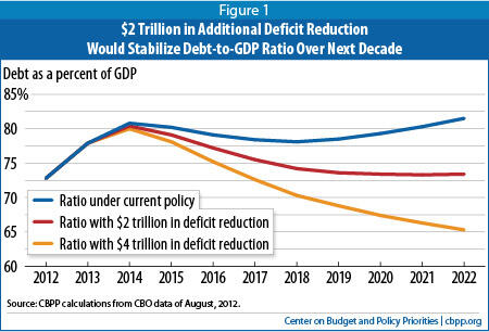
Though it would stabilize the debt over the coming decade, an additional $2 trillion in deficit reduction would not be enough to address the longer-term budget problem. In ensuing decades, the aging of America’s population and per-capita health care costs that are likely to rise faster than per-capita GDP will put considerable pressure on federal health and retirement programs, returning the budget to an unsustainable path of rising debt as a share of the economy. Nevertheless, by stabilizing the debt for the next decade, an additional $2 trillion in savings would give experts and policymakers time to figure out how to slow the growth of health care costs throughout the U.S. health care system without impairing the quality of care. An additional $4 trillion of deficit reduction over the next decade would, in contrast, result in a declining debt ratio (as Figure 1 shows) but would require policymakers to make decisions today on policies, particularly in health care, where desired solutions remain elusive.
There are major unknowns in the health arena. Health care cost growth has slowed appreciably over the past two years. Experts don’t yet know whether this slowdown is permanent or only temporary, and the answer will affect both the magnitude of the long-term fiscal problem and the extent to which further slowing of health-care cost growth is required.
More fundamentally, we currently lack needed information on how to slow health cost growth without reducing health care quality or impeding access to needed care. Demonstration projects and other experiments to find ways to do so are now starting, some of them government-funded and others being undertaken in the private sector. By later in the decade, we should have substantially more knowledge of what works and what doesn’t. Taking major policy action in this area now before we have the necessary knowledge and experience risks putting us on a course that could fail to restrain health costs, compromise health care quality, or harm substantial numbers of sick or otherwise vulnerable individuals. An additional $2 trillion in deficit reduction would, by stabilizing the debt for the coming decade, buy time to find answers to these important questions.
If the goal is $2 trillion in additional savings (or some other such number) over ten years, policymakers will need to determine not only how to get there but at what pace. They could phase in the savings gradually so the savings grow in size over a number of years, or they could have the full programmatic effect of the savings start in the first year. With the economy still recovering from the Great Recession, a gradual path to deficit reduction makes more economic sense; it also would produce more long-term deficit reduction because, under such an approach, the amount of deficit reduction would be larger in the final years of the coming decade than under an approach in which the cuts start immediately. (For more on why the path matters, see Box 2 on p. 7.)
In calculating that $2 trillion in additional deficit reduction is needed to stabilize the debt, we use a current-policy baseline that is consistent with the current-policy baselines constructed by other budget analysts and institutions. Specifically, it assumes that policymakers: extend all of the tax cuts that are due to expire at year-end (except for the “tax extenders” — see below); freeze Medicare reimbursement rates for physicians at current levels; phase down war funding over the next few years; and not allow the scheduled across-the-board spending cuts (“sequestration”) to occur. Further, the baseline assumes that policymakers will not continue (or will offset the costs of continuing) a series of special tax provisions generally related to business income that are often referred to as the “normal tax extenders,” most of which expired at the end of 2011. (See Appendix I for more details on the baseline.)
While CBO assumes continuation of the tax extenders in its “alternative fiscal scenario,” both the Obama Administration and the Bowles-Simpson fiscal commission do not assume continuation of these measures in their budget baselines (or assume that policymakers would offset the costs of any “extenders” that they continued). The Committee for a Responsible Federal Budget treats the tax extenders the same way, as does our analysis. Whether or not one assumes that these measures continue doesn’t change the size of the near-term fiscal challenge. If a budget baseline assumes that policymakers continue these measures without offsetting the cost, the savings needed to stabilize the debt grow from $2 trillion to $3 trillion — but policymakers can return it to $2 trillion by simply not continuing these tax breaks or paying for those they do continue. (See Appendix II for more discussion of the treatment of the tax extenders.)
The $2 Trillion Target
While $2 trillion in additional deficit reduction is needed to stabilize the debt over the coming decade, that does not mean $2 trillion in policy savings are required. That’s because policy savings also generate savings in interest payments on the debt.
Policymakers could achieve $2 trillion with about $1.74 trillion in revenue increases and program cuts, which would generate about another $260 billion in savings in interest payments. (See Table 1.) The $2 trillion in savings would reduce the debt as a share of GDP from a peak of 80 percent in 2014 to 73 percent by the end of the decade, given the timing of deficit reduction that we have modeled. (See Figure 1.)
| Table 1 Additional Policy and Interest Savings over Ten Years, and Debt in 2022 In billions of dollars | ||||
| Policy savings | Interest savings | Total savings | Debt in 2022 (% of GDP) | |
| Current policy | 0 | 0 | 0 | 81.6% |
| $2 trillion in additional deficit reduction | 1,740 | 260 | 2,000 | 73.4% |
Many policymakers and pundits assume that the President and Congress must find $4 trillion in savings to address the deficit problem. Indeed, the $4 trillion figure has assumed an almost mythical status, with an importance that extends beyond any consistent analysis of the nation’s fiscal challenge. Importantly, the figure has no set meaning: people come to it from a variety of angles, apply the figure to a variety of budget baselines, and differ in the extent to which they count already-enacted savings.
The $4 trillion figure likely has its origins in the December 2010 Bowles-Simpson report, which proposed nearly $4 trillion of deficit reduction. But over the nearly two years since that report was released, the ten-year window for assessing budget plans has shifted, policymakers have achieved $1.7 trillion of deficit reduction by placing limits on discretionary spending, projections of the economic and fiscal outlook have improved significantly, and the “plausible” budget baseline used by the Bowles-Simpson commission has been supplanted in budget deliberations by a current-policy baseline like the one we use. As Figure 1 shows, an additional $4 trillion of deficit reduction measured relative to a current-policy baseline — which is the likely benchmark against which deficit-reduction proposals in the lame duck session will be assessed — provides substantially more deficit reduction than is needed to stabilize the debt, resulting in the debt-to-GDP ratio declining markedly over the decade.
The $2 trillion figure, which may appear smaller than some assumed was necessary to stabilize the debt over the next decade, reflects two basic facts:
- Substantial savings were enacted in 2011. The President and Congress enacted $1.7 trillion in savings last year (including interest savings), first through reductions in appropriations levels in March and April 2011, followed by the enactment in August 2011 of the Budget Control Act (BCA), which set annual caps on funding for “discretionary” programs (the non-entitlement programs that are funded through the appropriations process) for each of the next ten years. CBO’s estimate of the total amount of discretionary spending under the BCA caps from 2013-2022 is $1.5 trillion below the CBO baseline estimate at the end of 2010 of discretionary spending for this same period. This $1.5 trillion spending reduction produces more than $200 billion in interest savings, for total deficit reduction of $1.7 trillion.[1] The resulting reductions in discretionary programs will be large. Under the BCA caps, both defense and non-defense discretionary funding will decline by the end of the coming decade to a lower percentage of GDP than any on record, with data going back to 1976.
The end of 2010 is the appropriate starting point for measuring the amount of deficit reduction achieved; the Bowles-Simpson and Rivlin-Domenici plans were issued in late 2010 and are often viewed as the benchmarks against which to measure other plans.[2] The BCA’s discretionary caps have achieved about 70 percent of the savings in discretionary spending that Bowles-Simpson proposed, and they substantially exceed the savings in discretionary spending that the Rivlin-Domenici plan included. When comparing other deficit-reduction plans with Bowles-Simpson or Rivlin-Domenici, we and other analysts would be remiss if we did not include the enacted savings in discretionary spending.[3]
An additional $2 trillion in deficit reduction would, when combined with this $1.7 trillion in enacted savings, produce $3.7 trillion in total deficit reduction, relative to the policies in place at the start of 2011. This $3.7 trillion in total deficit reduction would be a notable achievement. As noted, it would entail policy savings that total 1.8 percent of GDP by the fifth year (2018), which would rank it alongside the landmark bipartisan budget agreement of 1990, which also included policy savings that totaled 1.8 percent of GDP by its fifth year. The total would exceed the 1993 budget agreement, which included policy savings that totaled 1.6 percent of GDP by the fifth year. - CBO’s forecast has improved. CBO’s August 2012 baseline reflects somewhat brighter economic and budgetary projections for the next decade than earlier CBO forecasts did. This makes the job of stabilizing the debt over the next decade somewhat less difficult to achieve. Using a baseline that assumes policymakers will continue current tax and spending policies, the projected debt in 2022 is almost $3.2 trillion lower under CBO’s August 2012 baseline than CBO’s August 2010 baseline would have shown if extended to 2022. Roughly three-fifths of the $3.2 trillion improvement is due to the reductions in discretionary funding enacted in 2011. But quite apart from those savings, CBO’s debt projections are about $1.5 trillion less pessimistic than the comparable projections made two years ago for economic and technical reasons. Some $750 billion of this improvement has come recently; the underlying current-policy projections associated with CBO’s August 2012 baseline are better than those in CBO’s March 2012 baseline by that amount.
The budget picture has also benefited from the nation’s decision to wind down military operations in Iraq and Afghanistan, which is producing substantial savings. These savings do not, however, factor into estimates of the amount of deficit reduction needed to stabilize the debt because our analyses and the Bowles-Simpson, Rivlin-Domenici, and other plans consistently assumed such savings in their baselines. Nevertheless, savings from winding down military operations have occurred somewhat faster than assumed in 2010 baselines and so contribute almost $100 billion to the total $3.2 trillion improvement in 2022 debt under current policy that we discuss above.
The Longer-Term Challenge
Beyond the next decade, rising health care costs and the aging of the baby boom generation are the two major factors behind projected longer-term federal deficits. Future health costs are highly uncertain, however, and we have much more to learn about how best to slow their rate of growth without compromising health care quality or impeding access to needed care.
The growth of both public and private health costs has slowed in the past few years. Spending for Medicare — the largest federal health program — grew by only 3.2 percent in fiscal year 2012, CBO has reported,[4] as compared with average growth of 6.7 percent a year from 2007 through 2011. CBO’s latest projections of total Medicare spending under current policy over the coming decade are about $400 billion below the projections CBO made two years ago. It’s too early to tell if this slowdown is permanent or temporary, but the slowdown has nevertheless produced a reduction in projected Medicare spending over the coming decade.
Over the longer run, policymakers will almost certainly have to take further significant steps to curb the growth of costs throughout the U.S. health care system as we learn more about how to do so effectively.
Box 1: Why the Debt Ratio Matters
The debt ratio — the debt held by the public as a share of GDP — should rise only during hard times or major emergencies and should fall during good times. That allows the ratio to remain stable over the business cycle as a whole and enables the government to combat recessions through tax cuts and spending increases (and to address human misery during bad times).
The debt ratio cannot rise forever. If it did, that would shrink the amount of national saving available for private investment, ultimately impairing productivity growth and, in turn, living standards. Alternatively, if foreign capital offsets the shortfall in domestic capital, the profits from that investment will go abroad; either way, U.S. living standards would suffer. In a crisis, international credit markets might refuse to lend to the U.S. public or private sectors at a reasonable price. These problems would occur if the debt ratio became too high. While no one knows what “too high” means for the United States, a debt ratio that rises in both good times and bad will become increasingly problematic.
That’s why the minimum appropriate budget policy is to ensure that the debt ratio does not rise during normal economic times. Achieving that would require shrinking deficits to below 3 percent of GDP. In the illustrative $2 trillion deficit reduction path shown in Figure 1, deficits average 2.5 percent of GDP from 2018 through 2022.
A $2 trillion deficit reduction package would stabilize the debt at about 73 percent of GDP by 2018. Some analysts prefer a lower debt ratio, such as 60 percent of GDP, a goal that the European Union and the International Monetary Fund adopted some years ago. No economic evidence supports this — or any other — specific target, however, and IMF staff have made clear that the 60 percent criterion is an arbitrary one. In addition, even if such a target were the best one before the recent severe economic downturn pushed up debt substantially in most advanced countries, it would not necessarily be an appropriate target for debt over the next ten years, given the severity of the downturn and continued economic weakness. The critical goal now is to stabilize the debt in the coming decade.
Stabilizing the debt during this decade will not permanently solve our fiscal problems; policymakers will need to enact additional deficit reduction for the long term. But it would represent an important accomplishment.
It also should be noted that there can be risks in policymakers setting their sights too high. If the political obstacles facing a much larger deficit-reduction package are too great, then insistence on a package that goes well beyond stabilizing the debt could lead either to failure — i.e., to enactment of no deficit reduction package — or to a package that provides false security because it is dominated by budget gimmicks that don’t actually reduce our long-term deficits but merely appear to do so.
Box 2: Why the Path of Deficit Reduction Matters
Optimally, policymakers would enact the needed additional deficit reduction shortly but not fully phase it in until later, say 2016. This is a time when sooner is not better.
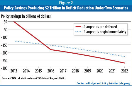
Figure 2 shows two paths for policy savings, each of which would produce $2 trillion in deficit reduction through 2022. The blue, dashed line has deficit reduction starting immediately. The red, solid line initially displays smaller cuts but ultimately displays deeper cuts. That’s the scenario represented by the red line in Figure 1, which entails smaller cuts upfront and deeper cuts in years after that.
The red-line scenario is better for the economy in the short run because, relative to current policy, it does not entail program cuts or revenue increases in 2013, when the economy will still be weak. It’s also better in the long run because it ultimately involves more real deficit reduction. While the two scenarios each produce $2 trillion in deficit reduction over the first decade, the trajectory reflected in the red line produces nearly $6 trillion in deficit reduction over the second decade while the blue-line trajectory produces slightly more than $5 trillion.[5]
Appendix I:
Current Policy and Methodology
Current policy. We measure deficit reduction from a current-policy baseline, constructed using estimates published by CBO in its August 2012 baseline update, rather than from CBO’s current-law baseline. In its current-law baseline, CBO follows the definition of a baseline set forth in §257 of the Balanced Budget and Emergency Deficit Control Act of 1985 as amended [2 U.S.C. 907]. That definition specifies (with exceptions) that any provision of tax law or of an entitlement program that is scheduled to change in the future, including provisions scheduled to expire, should be assumed to change on schedule. However, that legal definition is now sufficiently unrealistic that almost every budget analyst modifies the current-law baseline so it more closely represents current policy — that is, the budget laws as they apply in 2012. We modify CBO’s current-law baseline in the following ways.
- SGR. We assume that Medicare reimbursement rates for physicians will remain frozen over the decade rather than dropping precipitously, as otherwise required by the misnamed “sustainable growth rate” provision of current law.
- Sequestration. We assume that the sequestration scheduled to occur on January 2, 2013, and remain in effect through 2021 — required under current law because of the failure of last fall’s Select Committee on Deficit Reduction (the “Supercommittee”) — will not occur.
- War funding. We assume that funding for the Iraq and Afghanistan wars will phase down over the next few years, consistent with a level of 45,000 troops in Afghanistan by 2015 and thereafter, using figures supplied by CBO in its August 2012 baseline report.
- Expiring tax provisions. In general, we assume the continuation of all expiring tax provisions except the 2010 temporary payroll tax cut. This is also the approach to expiring tax provisions taken by CBO in its alternative fiscal scenario and by the Tax Policy Center in its current-policy baseline.[6]
However, for purposes of this analysis and our recent analysis of the Bowles-Simpson deficit-reduction plan (see footnote 2), we do not assume continuation of the so-called normal tax extenders, in order to make our analysis conceptually similar to deficit reduction as it is spoken of when comparisons are made to the Bowles-Simpson plan. The Committee for Responsible Federal Budget takes the same approach in its baseline. Appendix II provides further discussion of this matter.
To be more precise about our approach to expiring tax cuts, our baseline assumes continuation of the tax cuts enacted in 2001, 2003, and 2009 and then extended for two years in 2010. This assumption covers both the “middle-class” and the “upper-income” portions of the so-called Bush tax cuts. This assumption also includes the continuation of section 179 expensing, which was part of the 2003 tax cuts, as well as the creation of the American Opportunity Tax Credit and increases in the Child Tax Credit and the Earned Income Tax Credit enacted in 2009.
Method for modeling hypothetical deficit reduction. Relative to the current-policy baseline described above, we build four hypothetical deficit-reduction paths. For each path, we assume that deficit reduction will start in fiscal year 2014 and be fully phased in by 2016. We select a dollar amount of policy savings for 2014 and assume it will double in 2015, triple in 2016, and grow in nominal terms by 6.7 percent per year thereafter. We choose 6.7 percent because that is the unweighted average annual growth rate of revenues and Medicare in the current-policy baseline. To the extent that the bulk of additional deficit reduction comes from revenues and health entitlements, it is reasonable to expect that, once the policies in question are fully phased in, the savings will grow at the same rate as the baselines of these programs. Finally, we use CBO’s August 2012 interest rates to calculate the interest savings that will occur as a result of the policy savings we assume.
More precisely, given a target for total deficit reduction over ten years, a starting figure for policy savings in 2014 is sought that produces the desired ten-year total results. Table 2 shows the year-by-year policy and interest savings associated with the hypothetical $2 trillion deficit-reduction path used in Figure 1 and Table 1.
| Table 2 Policy Savings and Interest Savings in the Hypothetical $2 Trillion Path In billions of dollars | |||
| Fiscal year | Policy savings | Interest savings | Total savings |
| 2013 | 0 | 0 | 0 |
| 2014 | 61 | 0 | 61 |
| 2015 | 121 | 1 | 122 |
| 2016 | 182 | 5 | 186 |
| 2017 | 194 | 11 | 205 |
| 2018 | 207 | 23 | 230 |
| 2019 | 221 | 35 | 256 |
| 2020 | 236 | 47 | 283 |
| 2021 | 252 | 61 | 312 |
| 2022 | 269 | 75 | 344 |
| Total | 1,741 | 259 | 2,000 |
Finally, in calculating the resulting debt as a percent of GDP and displaying it in Figure 1, we smooth the path of deficits and debt to avoid certain meaningless bumps in the path. Four programs (SSI, veterans’ compensation and pensions, military retirement, and Medicare payments to Medicare Advantage and Part D plans) include a provision whereby, if the scheduled monthly payment would fall on a weekend, it is accelerated to the prior Friday. When October 1 (the first day of the fiscal year) falls on a weekend, the payment normally made on that date instead occurs on September 29 or 30, which is in the prior fiscal year. As a result, while most fiscal years include 12 such monthly payments, a few include 11 or 13. This makes deficit and debt figures appear bumpier than they really are (and happens to overstate the deficit and debt in 2022 by $44 billion because that year includes 13 of such monthly payments). To make the resulting debt levels and path more meaningful, we assume 12 monthly payments in each fiscal year. We build this assumption into the baseline so that this smoothing does not count as deficit reduction or a deficit increase.
Appendix II:
Current Policy and the “Normal Tax Extenders”
A large series of special tax provisions, generally relating to the treatment of business income, are regularly continued for a year or two at a time. The Research and Experimentation tax credit is the most prominent. Most of these special provisions expired at the end of 2011 but it is widely believed they will be reinstated, retroactive to the beginning of 2012. The continuation of the normal tax extenders (NTEs) is assumed in CBO’s alternative fiscal scenario and the Tax Policy Center’s current-policy baseline, as well as the Concord Coalition’s current-policy baseline.
We do not assume their continuation in this current-policy baseline, however, largely because the Bowles-Simpson commission and the Administration did not continue them in their current-policy baselines. (The Committee for a Responsible Federal Budget has adopted the same approach in its current-policy baseline.) We think it will be less confusing if we maintain broad comparability with their baselines. (For this reason, we also did not assume the continuation of the NTEs in our analysis of the original Bowles-Simpson plan, referred to in footnote 2.)
There is a case, however, for treating the NTEs like any other expiring tax provision that was clearly intended to be permanent. What if we had used a current-policy baseline in which the NTEs were assumed to be continued? Given the history of the last few decades, that would be a defensible way of envisioning current policy.
Under such a baseline, the starting level of revenues would be $848 billion lower over the period 2013-2022 and interest costs would be almost $150 billion higher. Thus, the current-policy baseline deficit would be almost $1 trillion higher over ten years. Consequently, stabilizing the debt would require $3 trillion, not $2 trillion, in deficit reduction. By the same token, however, one could achieve the “extra” trillion in needed deficit reduction by allowing the NTEs to expire or paying for those NTEs that policymakers choose to extend.
In short, it makes no difference to the bottom line if you start with a baseline in which the NTEs have expired and then find $2 trillion in additional deficit reduction, or if you start with a baseline in which the NTEs are continued and then find $3 trillion in deficit reduction, of which up to $1 trillion could be achieved by the expiration of some or all of the NTEs or by paying for those NTEs you chose to continue.[7] The resulting levels of revenues and debt are the same either way.
The key point, however, is that everyone — policymakers, the press, the public, and the business community — must be aware of what is in the baseline. If the baseline does not assume the continuation of the NTEs (as ours does not), then a) policymakers cannot count the expiration of any NTEs as deficit reduction as they try to achieve at least $2 trillion in deficit reduction, and b) policymakers cannot achieve $2 trillion in deficit reduction and then, later in the year, ask that the NTEs be continued without being paid for.
End Notes
[1] See Richard Kogan, Congress Has Cut Discretionary Funding by 1.5 Trillion over Ten Years, Center on Budget and Policy Priorities,September 25, 2012, https://www.cbpp.org/sites/default/files/atoms/files/9-25-12bud.pdf .
[2] For an analysis of the components of the Bowles-Simpson plan over the 2013-2022 period, measured from the baseline used in this report, see Richard Kogan, What Was Actually in Bowles-Simpson — And How Can We Compare it With Other Plans?, Center on Budget and Policy Priorities, October 2, 2012, https://www.cbpp.org/sites/default/files/atoms/files/10-2-12bud.pdf.
[3] We explain the importance of counting all the steps in a deficit reduction journey in “Of Zeno’s Dichotomy Paradox, “Takers,” and Deficit Reduction,” Off the Charts blog, February 16, 2012, http://www.offthechartsblog.org/of-zenos-dichotomy-paradox-takers-and-deficit-reduction/.
[4] This figure subtracts premiums paid by beneficiaries and corrects for shifts in the timing of payments. Congressional Budget Office, Monthly Budget Review, Fiscal Year 2012, October 5, 2012, http://www.cbo.gov/sites/default/files/cbofiles/attachments/2012_09_MBR.pdf.
[5] The estimates in this analysis are static in the sense that the deficit reduction modeled in Figures 1 and 2 is not assumed to speed up or retard economic growth. The discussion above, however, suggests that different paths to deficit reduction carry both economic risks and rewards. For example, if deficit reduction impairs growth (in the short run by withdrawing needed demand from a weak economy, or in the long run by underfunding public investment), then GDP will be lower than CBO projects and the same dollar level of debt will produce a higher debt-to-GDP ratio. The converse is also true, so that if done wisely, the deficit reduction modeled in this analysis would likely produce lower debt ratios than shown in Figure 1 and Table 1.
[6] For a table detailing these tax and other adjustments to CBO’s current-law baseline, see Kathy A. Ruffing and James R. Horney, Downturn and Legacy of Bush Policies Drive Large Current Deficits, Center on Budget and Policy Priorities, updated October 10, 2012, https://www.cbpp.org/sites/default/files/atoms/files/10-10-12bud.pdf.
[7] On August 1, 2012, CRFB issued a statement strongly urging Congress to offset the cost of any of the NTEs it does continue. See http://crfb.org/sites/default/files/Dont_Put_the_Extenders_on_the_Nations_Credit_Card.pdf.
More from the Authors