The Critical Importance of an Independent Central Bank
Testimony by Jared Bernstein, Senior Fellow,
Before the House Committee on Financial Services: Subcommittee on Monetary Policy and Trade
Chairman Barr and Ranking Member Moore, thank you for the opportunity to testify today.
My testimony begins with a discussion of Title X of the Financial CHOICE Act, which would undermine the independence and flexibility of the Federal Reserve, one of the few national institutions that has, in recent years, worked systematically and transparently to improve the economic lives of working Americans. By aggressively rolling back necessary financial oversight, much of the rest of the CHOICE Act would be an act of economic amnesia, one that would raise the likelihood of a return to underpriced risk, bubbles, bailouts, and recession — while Title X of the Act would hamstring the central bank’s ability to respond to the problems engendered by the rest of the Act.
My testimony also makes the following points:
- The evidence shows that monetary policy as practiced by the Federal Reserve, while not perfect, significantly boosted jobs and growth in the Great Recession and the recovery that followed, without generating market distortions.
- While monetary policy was often helpful in terms of pulling forward the current expansion, fiscal policy, starting around 2010, was uniquely austere and counter-productive, leading to job loss and a weaker expansion.
- There are policy measures that could be pursued to help those left behind in the current economy, including both monetary and fiscal policies. In the latter case, however, policies in budget plans from President Trump and House Republicans, along with the repeal of the Affordable Care Act, would hurt, not help, disadvantaged workers.
The Impracticalities and Dangers of an Overly Rules-Based Federal Reserve
It is widely recognized across advanced economies that for central banks to be most effective in carrying out their mandates, they must be politically independent. Of course, the Federal Reserve must meet the broad mandates Congress legitimately sets for it, which in the U.S. case is aptly summarized as full employment at stable prices. But any micro-managing of how the Fed meets its mandates by those who hold political office raises the specter of politicizing the bank’s actions. As current Fed chair Janet Yellen recently wrote, the “framework” wherein the Fed independently pursues its statutory goals “is now recognized as a fundamental principle of central banking around the world.”[1]
Title X of the Choice Act (this title was formerly the stand-alone Fed Oversight Reform and Modernization Act of 2015) would violate this critical norm.
A remarkable aspect of Title X is that it demands strict adherence to a policy rule, spelling out, in detailed language, a specific formula that corresponds to economist John Taylor’s 1993 eponymous “rule” and insisting that the Fed’s interest-rate-setting committee, the Federal Open Market Committee (FOMC), follow this rule in setting the federal funds rate (FFR) or face burdensome regulatory scrutiny.
The formula is specified as follows:
FFR = inflation + 0.5 * (output gap) + 0.5 * (inflation – 2%) + 2%
The “output gap” is specified as the percent deviation between actual and potential GDP, and inflation is the year-over-year rate of price growth. The first 2% is the Fed’s inflation target; the second is the variable that is these days called r*, which stands for the real interest rate at full employment and stable inflation that is neither expansionary nor contractionary.
To be clear, my objection is not to the utility of this rule, which is a sensible and intuitive formula (and a very important contribution to monetary policy). It essentially says that when inflation is above the Fed’s target the FFR should go up, and when output is below potential, the FFR should come down. When inflation is on target and output is at potential, the formula says the real FFR (nominal FFR – inflation) should be 2%, which is close to its long-term average (though I will soon show great variance around that average).
Its simplicity, along with the fact that certain versions of the rule generally track the actual movements in the FFR, makes the Taylor rule a standard tool for monetary policy makers. One of the first questions a monetary economist might ask in assessing the stance of Fed policy is, “where is the FFR relative to the Taylor rule?” However, while this might well be the first question, it should definitely not be the last.
For one, to say that the rule describes the past means neither that past rates were optimal nor that the rule’s output is appropriate for current or future conditions, a limit Taylor himself recognized in his seminal 1993 paper.[2] Therein, he noted that, to complement the information summarized in policy rules, central bankers needed to analyze “… several measures of prices (such as the consumer price index, the producer price index, or the employment cost index) … expectations of inflation as measured by futures markets, the term structure of interest rates, surveys, or forecasts from other analysts. . . .” Importantly, Taylor argued in that same paper that “there will be episodes where monetary policy will need to be adjusted to deal with special factors.” One such factor — the zero lower bound on the FFR — is particularly germane in this context.
Advocates of Title X might well inject at this point that the Act allows for such flexibility, but I strongly disagree. As I read the text of the bill, any time the FOMC strays from the “reference formula” specified in the Act (or a different version of the Taylor rule that had been previously sanctioned by the elaborate review process I’m about to describe), their rule change would be subjected to nine separate requirements, many of which are onerous enough to make deviation from the rule impractical.[3]
For example, within 48 hours of an FOMC policy meeting, the Fed chair must “describe the strategy or rule of the Federal Open Market Committee for the systematic quantitative adjustment of the Policy Instrument Target to respond to a change in the Intermediate Policy Inputs” (these are the variables in the rule). She must “include a function that comprehensively models the interactive relationship between the Intermediate Policy Inputs.” She must “include the coefficients of the Directive Policy Rule that generate the current Policy Instrument Target and a range of predicted future values for the Policy Instrument Target [the FFR] if changes occur in any Intermediate Policy Input.” And those are just three of the nine Title X requirements.
It is an astounding read from a Congress that claims to be invested in reducing red tape and complex regulation. It also creates a strong bias towards a solely rule-based approach that is, for reasons I now explain, increasingly unwise.
The Challenge in Identifying the Taylor Rule
Taylor’s work is important and justly influential. I assure the committee, however, that every single parameter in the Taylor Rule equation is fraught with uncertainty and questioned by the economics community. Note that:
- There isn’t consensus on the best inflation gauge. Taylor recommended the GDP deflator, but many contemporary applications of the rule use the PCE deflator, often the core version (excluding food and energy prices), as the Fed believes core PCE inflation to be the best predictor of future price growth.
- It’s unclear whether the coefficients should be 0.5. Former Fed Chair Ben Bernanke, in a recent piece that explores these very questions, argues that the coefficient on the output gap should be 1, not 0.5, as this formula more closely tracks the path of the FFR over the past few decades (Fed Chair Yellen has also made this point).[4] Researchers at the Kansas City Fed agree that “the equal weights on inflation and the output gap in the Taylor rule may not always be appropriate. While equal weights might be well suited for supply shocks, a greater weight on the output gap may be better suited for demand shocks.” [5] And recall that under Title X, the Fed would have to justify any such changes to their regulator at the Government Accountability Office (GAO).
- The output gap requires the input of unobserved variables that are increasingly difficult to nail down. The first such variable is potential GDP, meaning the level of GDP at full resource utilization, or, alternatively, the “natural” rate of unemployment, meaning the lowest jobless rate believed to consistent with stable inflation. There is considerable disagreement as to both the level of potential GDP and the natural rate of unemployment. Moreover, economists can only estimate these values these days within a wide confidence interval, meaning the formula above conveys a false sense of certainty. One recent analysis estimates that the current natural rate of unemployment is between a range that goes from 0 to 6 percent.[6]
- The level of another key unobserved variable in the rule, the “neutral” real FFR, is also a source of controversy among economists. This value is set at 2% in Taylor’s formula and in the “reference formula” of Title X (as noted, this variable is called r-star, or r*). But recent estimates of r*, such as those in Figure 1, show it to vary considerably over time, with some recent results near zero.
Figure 1 - The Fed’s explicit inflation target is 2%. But there is ongoing and increasing dissent on this point, with many economists now arguing that the Fed should raise its inflation target, in part because it would mitigate the risk of the FFR getting stuck at the “zero lower bound.” [7] Just last week, Chair Yellen recognized that this risk is greater than it has been in the past, pointing out “… that the economy has the potential where policy could be constrained by the zero lower bound more frequently than at the time when we adopted our 2% [inflation target].”[8] While Yellen noted that raising the target would engender both benefits and costs, to her credit, she clearly entertained the possibility that raising the inflation target could be necessary.
- The Fed must work with real-time data, which they must be able to informally adjust if known biases exist. For example, recent first-quarter GDP growth has appeared to be biased down, perhaps due to problems with seasonal adjustment. Failing to account for this bias could exaggerate the output gap. Pushing in the other direction, the unemployment rate has at times in recent years been biased down due to labor force exits, which in a rule-based approach could return a higher FFR that would itself be biased up. Under Title X, every time the Fed wanted to make adjustments to known biases, it would have to justify the adjustment to regulators at the GAO.
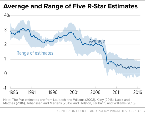
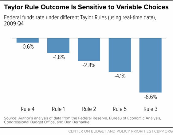
Table 1 takes these issues into account and presents results from many different versions of Taylor rules for two time periods, the depth of the Great Recession and now. First, note the sensitivity of the rule to the variable choices discussed above. Using real-time data that was available at the time, the rule as written in Title X hits its low point in the fourth quarter of 2009, when it recommended an FFR that was -1.8 percent. Switching to the core PCE deflator and plugging in an r* of zero takes the rule-based FFR to -2.8 percent (see row 2). Upweighting the slack coefficient leads to an FFR of almost -7 percent. If we stick with the “reference formula” but use unemployment instead of the GDP output gap, we get outcomes ranging from -0.6 to -4.1 percent. The range of results for these examples is shown in Figure 2.
| TABLE 1 | |||
|---|---|---|---|
| Rule No. | A Surplus of Taylor Rules | Low during Great Recession | Now |
| 1 | Standard Taylor Rule | -1.8% | 3.4% |
| 2 | (1) but with PCE core; r* = 0% | -2.8% | 1.1% |
| 3 | (2) but with slack coef = 1 | -6.6% | 0.6% |
| 4 | (1) but with u - u* instead of GDP gap | -0.6% | 4.0% |
| 5 | (3) but with u - u* instead of GDP gap | -4.1% | 1.7% |
| N/A | Actual FFR | 0.0% | 1.25% |
The differences in these results have huge policy implications. The Bernanke/Yellen Feds were running variants of these rules during the recession, and they appeared to lean towards the versions that bumped up the slack coefficient and plugged in a lower r*. Given the zero lower bound on the FFR, results like those in the table motivated them to turn to a set of other policies intended to lower longer-term interest rates, discussed in the next section of this testimony.
Turning to the second column in the table, the Title X reference formula returns an FFR of over 3 percent, which is at the high end of the range that current FOMC members forecast to be the long-run, equilibrium nominal rate that they will get to post-2019. By this measure, the current Fed is currently way “behind the curve.”[9] However, plugging a lower r* and weighting slack more heavily returns FFRs closer to the Fed’s current path.
This wide array of results raises numerous strong objections to the rules-based approach. First, the discretion of the Fed’s economists is essential in deciding which values to plug into the formulas. They should not have to consult regulators, as Title X would require them to, each time they tweak something. Second, they must have the leeway to decide how much weight to give the formula’s output given other economic and data dynamics. Consider today’s economy, where the job market is tight but wage growth is not accelerating and inflation has been decelerating. Though the standard rule would call for rapid removal of monetary accommodation, doing so would be incautious from the perspective of low- and middle-wage workers.
The combination of portentous choices to be made and politics is also a highly toxic mix, which is precisely why we do not want Congress micromanaging the Fed. The Fed is an independent, highly functional institution without an explicit political agenda; as such, it can go about its work in a much more analytical and less fractious political environment than that of today’s Congress. As a result, its approach is systematic, timely, and generally predictable, the last of which is important to markets.
Congress, conversely, is both much more political and less efficient. Partisan debates frequently cause deadlines to be moved back or missed. It would be an act of willful denial to not consider the problem of relative functionality — that of the Fed vs. Congress — when considering reducing the Fed’s independence and increasing Congress’s authority over their actions.
To be clear, none of that is to imply that the Fed’s monetary policy record is perfect, or that it doesn’t make costly mistakes. The Fed must not be immune from scrutiny and criticism; in fact, I myself recently administered a heavy dose.[10],[11] But that’s a far cry from giving Congress the power to reduce the central bank’s independence and effectiveness.
The Fed’s Large Scale Asset Purchases, a.k.a. Quantitative Easing
In late 2008, when the FFR first began bumping up against the zero lower bound and the economy was still very weak, the Fed announced that they would soon begin large-scale asset purchases, or LSAP, also known as quantitative easing, or QE. The purpose of this initiative, which involved the purchase of Treasury bonds and mortgage-backed securities (MBS), was to lower the cost of borrowing by targeting longer-term interest rates. How successful was the LSAP program and what, if any, costs did it impose on markets?
In a review of many studies of the impact of the LSAP on longer-term yields, John Williams finds that the asset purchases had “sizable effects on yields on longer-term securities,” but that the precise magnitudes of the effects were hard to tease out of the data.[12] That said, Williams notes:
The central tendency of the estimates [of the LSAP] indicates that $600 billion of [the] Federal Reserve’s asset purchases lowers the yield on ten-year Treasury notes by around 15 to 25 basis points. To put that in perspective, that is roughly the same size move in longer-term yields one would expect from a cut in the federal funds rate of 3/4 to 1 percentage point.
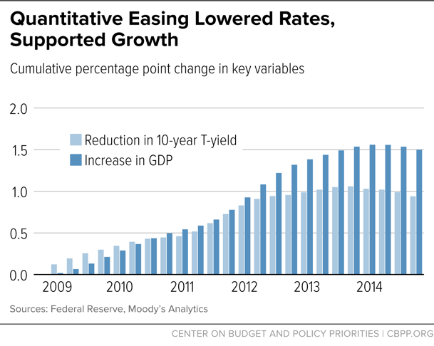
A simple statistical comparison of the impact of Fed rate changes on real GDP growth suggests a one-point decline in the FFR raises real GDP by about half-a-percent about 4-6 quarters later. Consistent with that result, Williams reports on research that finds the Fed’s LSAP program lowered the unemployment rate by one-quarter of a percentage point, which in today’s labor market amounts to 400,000 jobs. Alan Blinder and Mark Zandi, using a macro-model to score QE against a baseline with no such intervention, estimate that from 2009-14, QE lowered the 10-year Treasury rate by 1 percentage point and raised the level of real GDP by 1.5 percent (see Figure 3).[13]
As noted above, part of the Fed’s LSAP program involved purchasing MBS backed by the government-sponsored enterprises Fannie Mae and Freddie Mac. These asset purchases were intended to “reduce the cost and increase the availability of credit for the purchase of houses” at a time when the damage from the bursting of the housing bubble was constraining credit and thus economic activity in that critical sector. [14] While assessing the impact of the Fed’s MBS purchases is not simple, as many moving parts are in play, numerous analysts found that the program worked quickly to lower mortgage rates and help boost the ailing housing market.
Hancock and Passmore found, for example, that the Fed’s MBS purchases lowered mortgage rates by “roughly 100 to 150 basis points,” which they attribute to both the announcement of a “strong and credible government backing for mortgage markets” and the actual purchases themselves. They also report on other research, which finds “evidence of substantial announcement effects for the program, with estimates for the decline in interest rates ranging from 30 basis points to slightly over 100 basis points.” [15] John Williams of the San Francisco Fed has argued that the MBS purchases were the “most effective” part of the Fed’s asset purchase programs and that they “ended up having kind of the bigger bang for the buck than the Treasury purchases.”[16] Blinder and Zandi’s research underscores these findings. They report that, “within a short time” of this part of the LSAP initiative, “homebuyers with good jobs and high credit scores could obtain mortgages at record low rates, which helped end the housing crash.”[17]
The empirical evidence thus suggests that QE should be viewed as a useful tool when the FFR is constrained by the ZLB, though estimates of its impact are imprecise. However, a number of critiques have been offered against QE, and any potential downsides must be weighed against its benefits.
First, some critics worried QE would be highly inflationary. Yet the path of actual inflation has been consistently below the Fed’s 2 percent target rate, so that critique is easy to dismiss.
Second, some have argued that, by inflating asset values, and considering that financial assets are disproportionately held by the wealthy, QE exacerbated wealth inequality. The closest examination of this assertion is by economist Josh Bivens, who finds the claim to generally be ill-founded. First, and most importantly, any inequality-inducing impacts of QE must be weighed against the distributional impact of the benefits of monetary stimulus.[18] As Bivens puts it, “Stimulus that reduces unemployment disproportionately benefits low- and moderate-wage workers and leads to a compression of earnings.” Second, as the discussion of MBS above implies, QE made home loans more affordable, and Bivens notes that housing “is also the most democratically held asset across wealth classes.” Cogent arguments can be made that there are types of fiscal stimulus that are more progressive than LSAP, but as I stress below, there were periods in our recent history when needed fiscal stimulus was not forthcoming, and against this baseline of no positive fiscal impulse, Bivens correctly notes that, as long as the economy and the job market are below potential, “monetary stimulus is a strongly progressive policy.”
Third, some believe QE distorted financial markets by, for example, crowding out private investment in Treasuries and allocating too much credit to real estate. This critique too must be considered in the context of what else might have happened if the Fed had “given up” once the FFR hit the ZLB. Blinder and Zandi produce some of the most detailed analysis of such counterfactuals, modelling the impact on GDP, jobs, and unemployment of the policies to offset the last recession. Their “financial policy response” analysis goes beyond Fed policy, including the TARP and other credit enhancing programs. But presumably, all such interventions are relevant to those who object to alleged financial market distortions.
To try to isolate the impact of the financial system interventions, their counterfactual assumes no policy steps were taken to “shore up the financial system,” but fiscal policies, such as the Recovery Act, were implemented. They find that in 2014, the financial policy interventions had these effects:
- Real GDP was 5 percent higher than it otherwise would have been;
- The level of payroll employment was 4 million jobs above the alternative;
- The unemployment rate was 6.2 percent compared to the counterfactual level of 8.4 percent.[19]
It is incumbent on those making market-distortion arguments to show that avoiding such distortions would have been worth sacrificing these sorts of gains.
Another factor to consider against this critique is that the rules governing which securities the U.S. Fed can purchase are actually quite restrictive. As is by now widely known, the LSAP expanded the Fed’s balance sheet by over $4 trillion through purchases of Treasury bonds and MBS. Why did the Fed not allocate credit more widely, so as not to unduly influence yields in just these two asset classes? Because they had no choice (according to their read of their charter, at least). This restriction is unique among modern central banks: the banks of England, Japan, Canada, and Europe all have few restrictions on the types of assets they can purchase (though in some cases they must seek permission from regulators to go into, for example, equity markets).
Moreover, given actual market conditions at the beginning of the LSAP program, MBS purchases were warranted. Following the bursting of the housing bubble, private mortgage lending was severely constrained; even clearly credit-worthy borrowers in the prime market faced unusually tight lending standards. Given the private-sector’s pull-back in housing finance, the case for crowding-out distortions is weak. To the contrary, as the Fed is the “lender of last resort” in a credit crisis, its MBS purchases were well-timed and, as shown above, had their desired impact (with the caveat regarding the challenge of precise estimation).
In sum, the Fed’s LSAP was a necessary and helpful response to the deep recession of 2007-9. QE lowered longer-term interest rates, perhaps most importantly by delivering credit to the market for housing finance, at a time when the Fed’s short-term interest rate tool, the FFR, was bound by zero. Again, any claims of negative externalities must be evaluated against the benefits documented above.
Of course, as the economy closes in on full employment, the Fed has now officially announced its intentions to reduce its balance sheet by allowing matured loans to roll off (instead of rolling them over). However, they may want to consider one further potential benefit of their historically large balance sheet, one raised in recent work by former Fed governor Jeremy Stein et al. These authors document the increase in the demand for short-term debt, a demand typically met by overnight “commercial paper” — very short-term debt instruments that can be prone to dangerous volatility with big, systemic downside risk. By maintaining an historically large balance sheet (perhaps about half the size of their current holdings), Stein et al. argue that the Fed can provide much safer short-term debt, thereby weakening “the market-based incentives for private-sector intermediaries to issue too many of their own short-term liabilities.”[20]
This interesting and practical idea underscores my main recommendation to the committee regarding the Fed’s bond-buying program: when their main tool is tapped out, the central bank must be able to turn to other methods to boost the economy on behalf of businesses and households. Restrictions on these practices would be, like the extreme rules-based approach discussed above, a major mistake.
The One-Two Punch of Monetary and Fiscal Policy and the Dangers of Fiscal Austerity
While monetary policy in its various forms was highly effective in pushing back against the Great Recession, it takes both monetary and fiscal policy, working together, to generate a robust recovery. In fact, when he was Federal Reserve chair, Ben Bernanke made precisely this point in congressional testimony:
Although monetary policy is working to promote a more robust recovery, it cannot carry the entire burden of ensuring a speedier return to economic health. The economy’s performance both over the near term and in the longer run will depend importantly on the course of fiscal policy.[21]
There are at least three reasons for Bernanke’s assertion. First, while the LSAP had positive impacts as just described, once the FFR hits zero, the Fed’s firepower is constrained, especially given persistently lower interest rates in recent years (as reflected in Figure 1). Constrained potential for monetary stimulus raises the relative importance of fiscal stimulus.
Second, monetary and fiscal stimulus attack different parts of the problem in weak, demand-constrained economies. Monetary stimulus works largely through lowering the cost of borrowing, but people hurt by high unemployment may have too little income to take advantage of low interest rates. Relatedly, investors may see too little demand to take on new projects. To the extent that fiscal stimulus puts money in people’s pockets, say through infrastructure programs, direct job creation, temporary tax cuts, or increased safety net benefits (e.g., ramped up unemployment insurance), low- and middle-income people themselves can be more likely to take advantage of low borrowing costs, or to signal to investors through increased consumer demand that they should take advantage of low rates.
Third, monetary and fiscal policies interact in recessions to boost fiscal multipliers. If the economy is operating at full employment and government spending generates a positive fiscal impulse, the Fed may be likely to offset such spending by raising rates (this logic is consistent with the Taylor rules laid out above). But, as Bernanke’s comment above suggests, in a recession or weak recovery (note that the comment is from February of 2013), the Fed would not move to offset a positive fiscal contribution to growth. It is partly for this reason, per Blinder and Zandi’s analysis, that the “bang” for a dollar of fiscal stimulus is larger in recessions or weak recoveries. They estimate, for example, that each $1 boost in food stamps in 2009 would have been expected to raise GDP by $1.74, compared to $1.22 in 2015; comparable multipliers for state fiscal aid are 1.41 in 2009 versus 0.58 in 2015.[22]
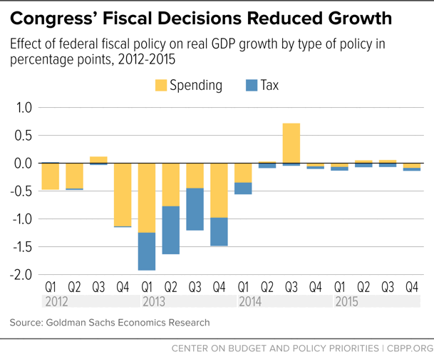
In fact, as Figure 4 shows, Bernanke had good reason to importune Congress for fiscal austerity — the reduction of fiscal support when private-sector demand is still too weak to support the needs of working families — in 2013. The bars show how much federal spending and tax decisions are estimated to have reduced GDP; the blue parts that year largely refer to the premature sun-setting of the “payroll tax holiday” that was helping to boost workers’ paychecks, while the yellow parts represent spending cuts driven by “sequestration.” As I’ve noted in prior testimony, the reduction shown (of 1.6 percentage points that year) cost us “over a million jobs lost based on historical relationships and about three-quarters of a point added to unemployment — at a time when the U.S. economy was still trying to recover from the residual pull of the Great Recession.”[23]
Another way to gauge the extent of budget austerity in recent years is to compare real, per-capita government spending across historical recoveries. Figure 5, from economist Josh Bivens, shows spending at all levels of government — federal, state, and local. Bivens notes that “…per capita government spending in the first quarter of 2016 — 27 quarters into the recovery — was nearly 3.5 percent lower than it was at the trough of the Great Recession. By contrast, 27 quarters into the early 1990s recovery, per capita government spending was 3 percent higher than at the trough, 23 quarters following the early 2000s recession (a shorter recovery) it was 10 percent higher, and 27 quarters into the early 1980s recovery it was 17 percent higher.”[24]

Combining the evidence in these figures with that of earlier sections suggests that it was fiscal, not monetary, policy that failed working people. Throughout the Great Recession and weak recovery, the Fed aggressively applied the tools at its disposal to pull the recovery forward and to try to offset the sharp demand contraction. Initially, from about 2009-10, stimulative fiscal policy was broadly complementary to that of the Fed, but shortly thereafter, fiscal impulse — the difference in fiscal support from one period to the next — turned negative, leaving the Fed to, in Bernanke’s words, “… carry the entire burden of ensuring a speedier return to economic health.”[25]
The costs of this damaging shift to austerity include the job losses (relative to a baseline where the fiscal impulse remained neutral) implied in Figure 4, but there is an even steeper cost as well. By prolonging the weak expansion and contributing to longer-term un- and underemployment than would otherwise have prevailed, austere fiscal policy likely triggered some degree of “hysteresis.” That is, cyclical damage from the last recession has likely led to a permanently lower level of real GDP relative to the pre-recession trend.
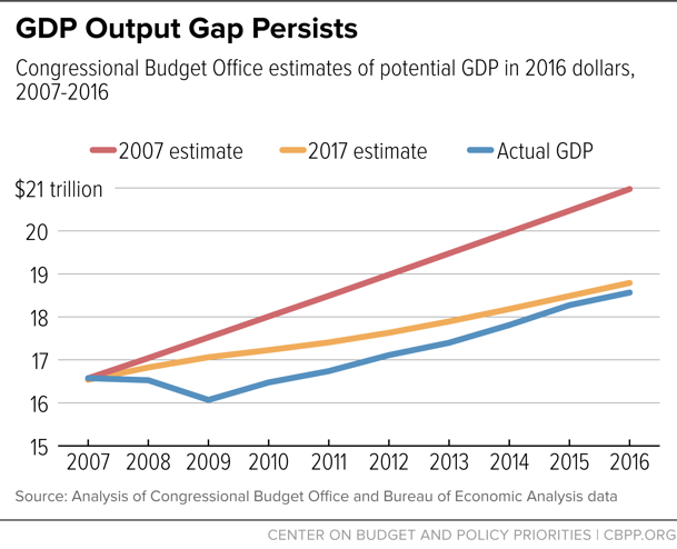
Figure 6 shows that CBO’s estimate of potential GDP is lower now than before the last recession. The gap in real dollars between today’s actual GDP and CBO’s downgraded potential, which it has just about caught up to, amounts to about $225 billion, or around $2,000 per household in the U.S. Slower trend economic growth and weaker productivity growth, both of which preceded the downturn, are likely partially responsible, but this downward revision is also certainly suggestive of scarring effects. Austere fiscal policy, by prolonging economic weakness, contributes to lasting economic losses.
Conclusion: What Would Helpful Fiscal and Monetary Policy Look Like Today?
As we enter year nine of the current expansion, there are steps that both monetary and fiscal policy makers can and should undertake.
Too often, congressional policies assume that all someone has to do to get a job is to want a job. But we know that, even as the U.S. economy closes in on full employment, labor demand remains weak for disadvantaged workers in various parts of the country. Measures to help those left-behind families include:
Targeted, direct job creation (fiscal): Direct job creation can take various forms. At the more interventionist end of the spectrum, the federal government provides a public service job for which it pays salary and benefits. Such employment could exist in fields ranging from infrastructure to education to child and elder care. A less interventionist approach is for the government to subsidize someone’s wage in a public, nonprofit, or private-sector job, an approach that was taken during the Great Recession — through the Temporary Assistance for Needy Families Emergency Fund (TANF EF) — and was quite successful, creating around 250,000 jobs. One careful study from TANF EF in Florida found that, relative to a control group, participants’ work and earnings went up not just during the program, but after it as well, suggesting lasting benefits.[26] A broader review of such programs shows we’ve done a lot more of this sort of job creation than is commonly realized, and well-designed programs in this space generate a big bang for the buck.[27]
In an effort to operationalize a direct job creation program, Ben Spielberg and I recommend that policymakers provide a dedicated funding stream (an “employment fund”) that can support job creation efforts and expand when and where the economy is weak.[28] Such a program would provide job creation for those left behind even in good times (whether due to discrimination, weak demand, or skill mismatches) and play a countercyclical role during recessions.
Targeting higher inflation or the price level (monetary): As noted above, economists increasingly recognize the risk of hitting the zero lower bound on the FFR. Having the Fed raise their inflation target or target the price level is increasingly regarded by economists as ways to avoid the recurrence of the lower bound problem.[29],[30] Establishing, for example, a 4 percent inflation target as opposed to the current 2 percent target would lead to higher nominal interest rates in recoveries, putting more distance between the nominal FFR and zero. Second, higher inflation implies lower real interest rates if we again do hit the lower bound (at an FFR of zero, the real interest rate is the negative of the inflation rate). Advocates of price-level targeting argue that requiring monetary policy makers to make up for periods of below-target inflation with above-target inflation would avoid the lower bound and, at the same time, clearly signal the Fed’s preferred inflation path. Of course, switching to a new target or to level targeting would not be costless, but any potential costs must be weighed against the potential for avoiding the lower bound problem and thus maintaining stable growth and unemployment targets.
While both these fiscal and monetary policy interventions would help address the economic concerns facing many Americans today and offset future periods of weak or recessionary growth, it is worth underscoring my fundamental conclusion that, in today’s hyper-partisan climate, the Federal Reserve remains a highly functional and efficient institution. I thus strongly urge the committee not to impose any sort of micromanagement over the Fed, as Title X of the Financial CHOICE Act would do. Of course, given the Fed’s influence in the domestic and global economies, their decisions and actions should be scrutinized by Congress and outside observers. But maintaining the operational independence of the central bank must remain one of this committee’s higher priorities.
End Notes
[1] Janet Yellen, Letter to Paul Ryan and Nancy Pelosi, November 16, 2015, https://www.federalreserve.gov/foia/files/ryan-pelosi-letter-20151116.pdf.
[2] John B. Taylor, “Discretion versus policy rules in practice,” Carnegie-Rochester Conference Series on Public Policy 39, 1993, pp. 195-214, http://web.stanford.edu/~johntayl/Papers/Discretion.PDF.
[3] H.R. 10 – Financial CHOICE Act of 2017, https://www.congress.gov/115/bills/hr10/BILLS-115hr10eh.pdf.
[4] Ben S. Bernanke, “The Taylor Rule: A benchmark for monetary policy?,” Brookings Institution, April 28, 2015, https://www.brookings.edu/blog/ben-bernanke/2015/04/28/the-taylor-rule-a-benchmark-for-monetary-policy/.
[5] Pier Francesco Asso, George A. Kahn, and Robert Leeson, “The Taylor Rule and the Practice of Central Banking,” Federal Reserve Bank of Kansas City, February 2010, https://www.kansascityfed.org/publicat/reswkpap/pdf/rwp10-05.pdf.
[6] Jared Bernstein, “Important new findings on inflation and unemployment from the new ERP,” On The Economy, February 22, 2016, http://jaredbernsteinblog.com/important-new-findings-on-inflation-and-unemployment-from-the-new-erp/.
[7] “Prominent Economists Question Fed Inflation Target,” Center for Popular Democracy, June 8, 2017, http://populardemocracy.org/news-and-publications/prominent-economists-question-fed-inflation-target.
[8] “Yellen Excerpt: Still ‘Highly Focused’ on 2% Inflation,” MNI Washington Bureau, June 14, 2017, https://www.marketnews.com/content/yellen-excerpt-still-highly-focused-2-inflation.
[9] “Economic projections of Federal Reserve Board members and Federal Reserve Bank presidents under their individual assessments of projected appropriate monetary policy, June 2017,” Federal Open Market Committee, June 13-14, 2017, https://www.federalreserve.gov/monetarypolicy/files/fomcprojtabl20170614.pdf.
[10] Jared Bernstein, “Why the Federal Reserve should not raise rates in June,” Washington Post, June 2, 2017, https://www.washingtonpost.com/posteverything/wp/2017/06/02/why-the-federal-reserve-should-not-raise-rates-in-june/?utm_term=.aca51f399a45.
[11] Jared Bernstein, “Is the Fed fighting an old war?,” On The Economy, June 15, 2017, http://jaredbernsteinblog.com/is-the-fed-fighting-an-old-war/.
[12] John C. Williams, “Monetary Policy at the Zero Lower Bound,” Brookings Institution, January 16, 2014, https://www.brookings.edu/wp-content/uploads/2016/06/16-monetary-policy-zero-lower-bound-williams.pdf.
[13] Alan S. Blinder and Mark Zandi, “The Financial Crisis: Lessons for the Next One,” Center on Budget and Policy Priorities, October 15, 2015, https://www.cbpp.org/research/economy/the-financial-crisis-lessons-for-the-next-one.
[14] Press Release, Board of Governors of the Federal Reserve System, November 25, 2008, https://www.federalreserve.gov/newsevents/press/monetary/20081125b.htm.
[15] Diana Hancock and Wayne Passmore, “Did the Federal Reserve’s MBS Purchase Program Lower Mortgage Rates?,” Federal Reserve Board Finance and Economics Discussion Series, January 2011, https://www.federalreserve.gov/pubs/feds/2011/201101/201101pap.pdf.
[16] Jeanna Smialek, “Fed’s Williams Prefers MBS Buying to ECB Tactics in Next Crisis,” Bloomberg, July 6, 2016, https://www.bloombergquint.com/global-economics/2016/07/06/fed-s-williams-prefers-mbs-buying-to-ecb-tactics-in-next-crisis.
[17] Blinder and Zandi.
[18] Josh Bivens, “Gauging the Impact of the Fed on Inequality During the Great Recession,” Brookings Institution, June 1, 2015, https://www.brookings.edu/wp-content/uploads/2016/06/Josh_Bivens_Inequality_FINAL.pdf.
[19] Blinder and Zandi.
[20] Robin Greenwood, Samuel G. Hanson, and Jeremy C. Stein, “The Federal Reserve’s Balance Sheet as a Financial-Stability Tool,” 2016 Economic Policy Symposium, Federal Reserve Bank of Kansas City, September 2016, https://scholar.harvard.edu/files/stein/files/jackson_hole_ghs_20160907_final.pdf.
[21] Ben S. Bernanke, “Semiannual Monetary Policy Report to the Congress,” Committee on Banking, Housing, and Urban Affairs, February 26, 2013, https://www.federalreserve.gov/newsevents/testimony/bernanke20130226a.htm.
[22] Blinder and Zandi
[23] “Testimony of Jared Bernstein, Senior Fellow, Before the House Budget Committee,” Center on Budget and Policy Priorities, June 17, 2015, https://www.cbpp.org/federal-budget/testimony-of-jared-bernstein-senior-fellow-before-the-house-budget-committee.
[24] Josh Bivens, “Why is recovery taking so long—and who’s to blame?,” Economic Policy Institute, August 11, 2016, http://www.epi.org/publication/why-is-recovery-taking-so-long-and-who-is-to-blame/.
[25] Bernanke, “Semiannual Monetary Policy Report to the Congress.”
[26] LaDonna Pavetti, “Subsidized Jobs: Providing Paid Employment Opportunities When the Labor Market Fails,” Center on Budget and Policy Priorities, April 2, 2014, https://www.cbpp.org/sites/default/files/atoms/files/4-2-14fe-pavetti.pdf.
[27] Indivar Dutta-Gupta, Kali Grant, Matthew Eckel, and Peter Edelman, “Lessons Learned from 40 Years of Subsidized Employment Programs,” Georgetown Center on Poverty and Inequality, Spring 2016, https://www.law.georgetown.edu/academics/centers-institutes/poverty-inequality/current-projects/upload/GCPI-Subsidized-Employment-Paper-20160413.pdf.
[28] Jared Bernstein and Ben Spielberg, “Preparing for the Next Recession: Lessons from the American Recovery and Reinvestment Act,” Center on Budget and Policy Priorities, March 21, 2016, https://www.cbpp.org/research/economy/preparing-for-the-next-recession-lessons-from-the-american-recovery-and.
[29] Josh Bivens, “Is 2 percent too low?,” Economic Policy Institute, June 9, 2017, http://www.epi.org/files/pdf/129551.pdf.
[30] John C. Williams, “Preparing for the Next Storm: Reassessing Frameworks and Strategies in a Low R-star World,” Federal Reserve Bank of San Francisco, May 8, 2017, http://www.frbsf.org/economic-research/publications/economic-letter/2017/may/preparing-for-next-storm-price-level-targeting-in-low-r-star-world-speech/.