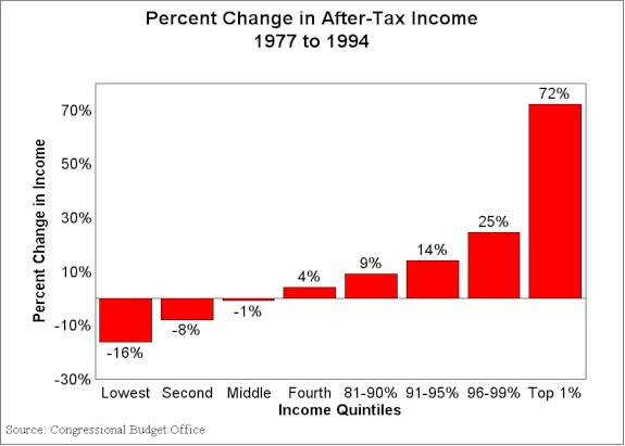
Table 1 shows the impact of the House legislation on average family income in each of eight income categories. The table reflects the impact of the legislation when the changes the legislation makes are fully in effect. This follows the standard approach the Joint Committee on Taxation and the Treasury Department have used in the past to estimate the distributional effects of tax cuts that phase in slowly or have delayed effective dates. Treasury and JCT have traditionally examined the distributional effects of such tax changes when the changes reach a steady state and are not still growing.

• The table shows that the net impact of the tax cuts and changes in entitlement programs would be to increase the average after-tax income of those in the middle 20 percent of the income distribution by $150. This increase, amounting to one-half of one percent of the average income of those in this income category, results from a modest tax reduction. Households in the next-to-the-top fifth of the income distribution would see their incomes rise an average of $240, or six-tenths of one percent of after-tax income, still a modest amount.

• All income groups except households in the top fifth of the income scale would either not receive a tax cut or receive a tax cut that, on average, constituted far less than one percent of their after-tax income.

• In contrast, those in the top income fifth would see their after-tax incomes rise an average of $2,570, or about three percent of their income. The top one percent of households, the nation's wealthiest, would secure the largest benefits. Their incomes would rise an average of $27,100, an increase equal to 6.1 percent of their already very large incomes.

• Figure 5 indicates that the legislation the House committees have approved would exacerbate the trends since the late 1970s toward widening income disparities. The families that have experienced the largest income increases since the late 1970s would fare very well under the bill, while those who lost income during this period would gain little or lose. As figure 5 illustrates, the poorest 20 percent of the population — which experienced an average decline of 16 percent in after-tax income between 1977 and 1994, after adjusting for inflation — would experience a small further decline in income as a result of the legislation.

• In contrast, the top quintile — which benefited from a 25 percent increase in average income, after adjusting for inflation — would garner another three percent gain from the tax and entitlement provisions modeled in this study.

The top one percent of the population — for which after-tax income has jumped 72 percent in inflated-adjusted terms since 1977 — would receive the largest income gains. The after-tax income of these households would rise an additional 6.1 percent of income.

When the tax cuts the House Ways and Means Committee has approved are in full effect, 40 percent of these tax reductions would accrue to the top one percent of the population. Some 60 percent of the tax benefits would go to the top five percent of the population. The average tax burden of the 20 percent of families with the lowest incomes, however, would not lessen.

The burdens of the cuts in entitlement programs that pay for these tax cuts (and help bring the budget into balance in 2002) are broadly shared. Nevertheless, these benefit reductions would be somewhat larger, when measured as a percentage of income, for those on the lower parts of the income scale than for those on the high end of the scale. The bottom 40 percent of households would lose an average of about one-half of one percent of their income due to the program reductions. Those at the top of the income scale would lose about one tenth of one percent of their income from the program changes.

Table 2 further illuminates these issues. It shows that the poorest 20 percent of the population receives 4.5 percent of the nation's total after-tax income. This segment of the population would, however, bear over 10 percent of the net entitlement reductions in the pending House legislation. Moreover, the poorest 20 percent of the population bore 64 percent of the benefit reductions in the 1996 reconciliation law. As noted, these households would not receive any benefits from the pending tax cuts.

By contrast, individuals in the top 20 percent of the distribution, who receive 49 percent of the nation's after-tax income, would get 80 percent of the tax benefits when the tax cuts are fully in effect. At the same time, they would shoulder only a modest share of the entitlement reductions in this year's legislation. They bore virtually none of the reductions included in last year's reconciliation law.

Combined Effects of 1996 and 1997 Reconciliation Legislation

The changes in income for the lower part of the income distribution look small, amounting to about 0.2 percent of income for the bottom two quintiles. This picture changes, however, when the effects of last year's reconciliation legislation are taken into account.

In 1995, Congress passed reconciliation legislation that included changes in Medicare and other non-means-tested entitlements, sweeping changes in low-income entitlement programs, and tax cuts. President Clinton vetoed the legislation. The legislation subsequently was divided; the 1996 reconciliation act — also known as the welfare bill — contained the reductions in the principal low-income entitlement programs other than Medicaid. When President Clinton signed the welfare bill, he pledged to change some of its most severe features. The fiscal year 1997 budget the Administration submitted earlier this year contained revisions in the welfare law. A portion of these are included in the legislation the House committees have approved.

Because the reconciliation legislation that is currently pending makes changes in the 1996 law, it makes sense to examine the distributional effects of the 1996 and 1997 reconciliation legislation combined. This is done in Table 3.

The table shows that households in the bottom fifth of the income distribution would lose an average of $420 a year — 4.6 percent of their after-tax income — when the combined effects of the 1996 and 1997 legislation are examined. Those in the next-to-the-bottom fifth would lose an average of $135. By contrast, those in the top fifth would gain an average of $2,560, or about three percent of income. Those in the top one percent of the population would receive an average increase in after-tax income of $27,000, equal to about six percent of their already very substantial income.

Figure 6 illustrates the overall impact on income of the 1996 and 1997 reconciliation legislation. The poorest 20 percent of the population would lose $9.2 billion. The second quintile would lose $2.8 billion. By contrast, the 20 percent of the population with the highest incomes would gain $58.8 billion.

The Effects of the Tax Provisions

Despite the inclusion of tax reductions such as the child tax credit and education tax cuts, the Ways and Means Committee tax bill has highly regressive effects. As Table 4 shows, the principal tax cuts that grow over time and eventually reach very large dimensions — the capital gains, IRA, and estate tax cuts — all provide more than 90 percent of their tax benefits to households in the top 20 percent of the income distribution. No more than 1.5 percent of the benefits from these three tax cuts would accrue to those in the bottom 60 percent of the income distribution.

These findings are consistent with those of various past studies and analyses. A recent Congressional Budget Office study has found that the top five percent of households receive approximately 75 percent of the capital gains income received in any given year.⁽¹⁾ Similarly, a Joint Tax Committee analysis conducted several years ago of the distributional consequences of a 1990 proposal to expand IRA eligibility in a manner similar to the Ways and Means Committee proposal found that 95 percent of the benefits from such a provision would accrue to the top 20 percent of households. The richest 4.5 percent of taxpayers would collect nearly one-third of the new tax benefits.⁽²⁾

Lower-income families would benefit little from the child tax credit. As Table 4 indicates, only one-half of one percent of the benefits the child tax credit provides would accrue to families in the lowest income quintile, even though 26 percent of all children under 18 are in that quintile. Under the Ways and Means Committee's plan, the child tax credit is limited to families that have federal income tax liability remaining after the Earned Income Tax Credit is computed. Families that do not owe income tax after the EITC is taken into account but have large remaining payroll tax liabilities would not be eligible for the credit. About six percent of the benefits from the credit would go to those in the top 20 percent of the population. (The credit phases out for married filers with two children between $110,000 and $150,000, with those above $150,000 ineligible for the credit.)

The tax package as a whole provides no benefits to individuals in the bottom 20 percent of the population and only a modest share of its benefits to the next 60 percent of the population. When the tax provisions reach full effect, the lion's share of the tax benefits accrue to the top 20 percent of the population; the top 20 percent of the population ultimately would receive 80 percent of the benefits.

Comparison of Republican and Democratic Revenue Packages

A budget that included a different mix of tax cuts would have a different impact on the distribution of income. Table 5 and Figures 7 and 8 examine the effects of the alternative tax package that Rep. Charles Rangel offered in the Ways and Means Committee. The table and figure compare the Rangel proposal to the Committee tax plan. The distributional impact of the Rangel proposal is nearly the inverse of that of the Committee bill.

• The Committee package provides no tax cut to the bottom fifth of households. For households in the next-to-the-bottom fifth, the Committee bill provides a modest tax cut equal to 0.5 percent of the average income of the households in this income category.

• The Committee bill provides a large tax cut, equal to 6.1 percent of income, to the top one percent of the population.

• The Rangel plan, on the other hand, provides a tax cut equal to 1.6 percent of income to the bottom income fifth and a tax cut that gradually decreases as a percentage of income as you move up the income ladder. The top fifth would get a small tax cut equal to 0.2 percent of income.

• The bottom three-fifths of the population would get a larger tax cut under the Rangel plan than under the Committee bill. The top two-fifths would receive a larger tax cut under the Committee bill. The differences would be greatest for those at the top of the income scale.

Figure 8

Another way to compare the proposals is to examine the share of the tax cuts each proposal provides to the various income groups. This is done in Table 5 and Figure 3.

• Under the Rangel plan, 15 percent of the tax cut benefits would go to the top 20 percent of the population. By contrast, these households would receive 80 percent of the tax cuts under the Ways and Means Committee plan.

• The Rangel plan would provide less than eight percent of its tax cuts to the top one percent of households. They would receive 40 percent of the Ways and Means Committee's tax cuts.

• At the bottom of the income spectrum, the bottom 40 percent of households would secure 38 percent of the tax cuts provided under the Rangel plan. They would get three percent of the tax cuts under the Ways and Means Committee plan.

One also can examine the proportion of tax cuts that each plan provides to those in the middle three-fifths of the income spectrum. The 60 percent of the population in the middle of the income spectrum would receive 70 percent of the Rangel tax cuts but only 21 percent of the Ways and Means Committee tax cuts. (Note: when fully in effect some time after 2007, the Ways and Means Committee tax cuts are more than twice as large in size as the Rangel tax cuts, which do not continue to grow in cost after 2007. As a result, households in the next-to-the-top quintile would get a larger dollar tax cut under the Ways and Means plan than under the Rangel plan even though they would receive a smaller percentage of the total tax cut under the Ways and Means plan.)

These large differences in the distribution of tax benefits under the two plans result primarily from two related factors. First, the tax provisions that principally affect high-income taxpayers — the capital gains, estate, IRA, and corporate alternative minimum tax provisions — are much smaller under the Rangel proposal than under the Committee bill. Second, the child tax credit is designed to bestow much more of its benefits on those in the bottom 40 percent of the income distribution under the Rangel plan than under the Committee bill.

In the Rangel plan, the child tax credit is refundable against payroll taxes. In addition, the child credit would be computed before, rather than after, the Earned Income Tax Credit is taken into account. Under the Ways and Means Committee version, the child credit is not refundable and is computed after the Earned Income Tax Credit is taken into account; a family whose EITC is larger than its income tax liability would receive no child tax credit even if it still owed payroll taxes not covered by the EITC.

In addition, under the Rangel alternative, the child credit would be fully phased out at $75,000 of income, and the deduction for education expenses would phase out at $100,000 of income. Under the Ways and Means bill, the child credit would not fully phase out for married filers with two children until income reached $150,000, and there would be no income limits on the education deduction. The education deduction would, in fact, provide more than twice as large a tax break to high-income families in the 31 percent, 36 percent, and 39.6 percent tax brackets as to middle-income families in the 15 percent tax bracket.

Methodology

The analysis presented in this paper provides an estimate of the distributional impact of both the tax provisions and the mandatory spending provisions in reconciliation legislation that House committees have passed in recent weeks. It also examines the impact of the Rangel tax proposal. To the degree possible, the methodology used to conduct this analysis follows the methodology used by the Congressional Budget Office in its analysis of the distributional impact of the 1990 budget agreement. The Office of Management and Budget used a similar methodology to estimate the distributional impact of the 1995 reconciliation bill.

Data from three different sources were combined to produce this analysis.

• Congressional Budget Office data on the distribution of income and the distribution of individuals throughout the income spectrum provide the backbone of this study.

• The impact of both the tax provisions the House Ways and Means Committee approved and the tax plan Rep. Rangel proposed was estimated by Citizens for Tax Justice, using the Institute for Taxation and Economic Policy microsimulation model.

• The impact of the mandatory spending changes was estimated by the Center on Budget and Policy Priorities using the Urban Institute's TRIM model.

Each of these components is discussed in detail below. For consistency, all three models used in this analysis employed the same definition of income and the same methodology of sorting individuals into income groups by adjusted family income.

Definition of Income

As noted, the definitions of before-tax and after-tax income used in the Center's study corresponds to those used by the Congressional Budget Office, with one exception. To the cash transfers included in the CBO definition, the Center has added near-cash transfers such as food stamps and housing subsidies. In measuring after-tax income, CBO accounts for all federal taxes but not state or local taxes (See the footnotes to Table 1 for the definition of income used in this study).

The CBO definition of income used here differs from that used by the Treasury Department and the Joint Committee on Taxation. Both Treasury and the JCT use an "expanded" definition of income that includes non-cash income, such as employer contributions to fringe benefits for pensions and health insurance. The JCT includes the health insurance value of Medicare but not Medicaid; Treasury includes the health insurance value of neither of these two programs. Treasury also includes in income the imputed rent on owner-occupied housing and some other types of non-cash income. In addition, Treasury and JCT use before-tax income, while the primary CBO definition of income used in this report measures after-tax income.

If the Treasury or JCT definition of income had been used in this analysis, it would not change the overall thrust of the results. Use of a broader measure of income would, however, have reduced the percentage change in family income that the tax cut and program changes are estimated to cause.

Sorting Individuals Into Income Groups

The first step in conducting this analysis involved the sorting of individuals into income groups. This analysis sorts individuals into income categories — principally income quintiles — based on their adjusted family income. Adjusted family income is a concept the Congressional Budget Office has developed; it is the standard method that CBO uses to sort individuals into income categories in all of CBO's distributional analyses. The adjusted family income approach adjusts each family's income by family size. In developing this approach, CBO recognized that a family of four with income of $15,000, for example, is much less well off than single individuals with the same income.

CBO measures a family's adjusted family income by dividing the family's before-tax income by the poverty line for that particular family size. (The poverty line varies by family size.) All individuals then are sorted by adjusted family income and divided into fifths, or quintiles. A quintile is defined such that each income fifth contains the same number of individuals (rather than the same number of families).

Neither the Treasury Department nor the Joint Committee on Taxation makes this adjustment. In Treasury and Joint Tax analyses, each quintile contains the same number of taxpaying units, not the same number of individuals. Their methods, while useful for some purposes, can be misleading when used to measure the distributional impact of tax or benefit changes. Consider a family of five with income of $18,000. This family's income is below the poverty line for a family of five. Yet under the Treasury Department methodology, this family would be "ranked" as having higher income than a family of two with income of $16,000, even though the second family has income that is over one and a half times the poverty line for a family of its size.

Furthermore, when families are sorted by family income under the methodology the Treasury Department and JCT use, individuals sorted into the bottom quintile are largely single, many of them elderly. Many of these individuals have incomes well above the poverty line. In contrast, families with children can fall into the second quintile even if their income is well below the poverty line. Because most "families" in the bottom quintile are single individuals, while most large families with children are in higher quintiles, the number of individuals and the type of individuals in each quintile varies substantially. A 1992 study showed that when families were sorted into quintiles on the basis of their income, without adjustment for family size, only 14 percent of the population and 14.5 percent of children were in the bottom quintile. The same study showed that when individuals were sorted by their adjusted family income, 20 percent of the population and 27.7 percent of children were in the bottom quintile.⁽³⁾

The same point can be illustrated by examining the number of personal exemptions for children that families in each income quintile could claim, using each of the two methodologies for classifying families into quintiles.

Under the methodology that the Treasury and JCT use, which does not adjust for family size when classifying families into quintiles, only 11.5 million children could be claimed by families in the bottom income quintile, while 23.8 million children could be claimed by families in the top quintile. Under the AFI methodology, this picture is nearly reversed — the number of children who could be claimed by families in the bottom quintile is 20.1 million, while the number who could be claimed for families in the top quintile is 11.6 million.

The Congressional Budget Office developed the adjusted family income approach to ranking individuals into quintiles to respond to these problems and to compare income growth over time for different segments of the population. The advantages of the AFI approach are two-fold. First, individuals are assigned to quintiles after appropriate adjustment for family size. As a result, the lowest quintile actually contains the poorest 20 percent of the population, when incomes are measured in relation to the poverty line. Second, because CBO has used this methodology to analyze changes in income over time, one can examine how the average income of each quintile has changed over time and how that compares to the changes in the average income of each quintile that would result from tax and spending provisions included in various budget proposals. For example, CBO analysis has shown that the after-tax income of the lowest quintile fell 16 percent between 1977 to 1994, after adjusting for inflation. Our analysis shows that the 1996 reconciliation law will cause a further reduction in average income of four percent for individuals in the lowest quintile. Neither the Treasury Department nor the Joint Committee on Taxation has published data on the changes over time in average income for the income groups.

There also is a disadvantage to the CBO approach — it is more difficult to explain simply. There is not a single set of income breaks for each quintile that can be expressed in dollar amounts, since the dollar breaks between the quintiles differ by family size.⁽⁴⁾ That makes it harder to explain simply how the quintiles are defined. Nevertheless, the advantages of this approach outweigh the disadvantages. At a minimum, policymakers should be aware of and utilize both approaches when considering the effects of policy changes on different income groups.

Because the composition of the population identified as falling into each quintile differs significantly between the two methodologies, the estimated distributional impact of the various tax provisions analyzed here also differs according to the methodology used. For example, as shown in Table 7, when families are sorted by the Treasury/JCT method, families in the next-to-the-top quintile receive a larger share of the benefits of the Rangel child tax credit than families in any other quintile. Families with children in this quintile appear to gain more than $7 billion, or 38 percent of the total tax cut the child credit provides, while those in the second quintile gain only $4 billion. When individuals are sorted by AFI, however, families in the second quintile gain the most — almost $6.5 billion — while families in the fourth quintile gain just $2.5 billion.

The AFI methodology also changes the measurement of how the proposed tax changes affect the very wealthiest families. Because the AFI methodology adjusts by family size, it tends to rank families with children lower in the distribution than the Treasury/JCT methodology does. As a result, there are few families with children in the top one percent of the distribution. Individuals sorted into the top one percent of the distribution under the AFI methodology are more likely to be older and less likely to have children. On the other hand, they are estimated to gain smaller benefits from the education tax breaks. By virtue of being older and less likely to have children — and therefore likely to have accumulated more wealth while no longer having to bear expenses for raising children — these individuals are more likely to be investors who will reap large benefits from the IRA, capital gains, and estate tax cuts. When the House Ways and Means Committee tax package is analyzed, the average tax cut for families in the top one percent of the distribution is estimated to be $24,785 when families are ranked by family income with no adjustment for family size, but $27,155 when individuals are ranked by AFI.

Distributional Analysis of the Tax Provisions

The distributional impact of each of the tax proposals included in the budget was estimated by Citizens for Tax Justice using the microsimulation model developed by the Institute for Taxation and Economic policy. The methodology CTJ uses for determining the benefits that each income group will receive from specific tax changes is similar to that used by the Treasury Department; in the past, CTJ distributional analyses have produced results similar to those the Treasury Department has produced. The CTJ methodology also is similar to the model that was used for many years by the Joint Committee on Taxation, although JCT methods have changed in the past few years.

In conducting this analysis, CTJ estimated the distributional impact of the following tax changes: the child tax credit, the indexing and phase-out of the Dependent Care Tax Credit, education tax cuts, changes to individual retirement accounts, capital gains tax cuts, the repeal of the alternative minimum tax, corporate tax cuts, estate tax cuts, and excise tax increases. This analysis covers more elements of the proposed tax package than do the distributional analyses issued by Treasury and JCT. Neither Treasury nor JCT estimated the distributional impact of estate taxes. In addition, Treasury did not estimate the distributional impact of the changes in excise taxes, while JCT omitted corporate tax changes from its distributional analysis.

The omission of estate taxes in other analyses does not necessarily reflect an inability to model those provisions. In 1993, the Joint Committee on Taxation published a methodology for estimating the distributional impact of changes in estate taxes.⁽⁵⁾ That methodology is used in this analysis.

The distributional impact of excise taxes was estimated by CTJ using the its consumption tax model, which is based on the Bureau of Labor Statistics' consumer expenditure survey. The estimates presented here on the distributional effects of the proposed changes in excise taxes are similar to the estimates of the Joint Committee on Taxation.

For purposes of this analysis, the impact of most tax cuts on family income are estimated when the tax cuts are "fully implemented." "Fully implemented" means that the impact of the tax changes is measured at the point when the provisions have been phased in fully and a sufficient time has passed for the provisions to reach their full cost.⁽⁶⁾ For example, the Individual Retirement Account provisions provide only a small tax benefit during the first few years because the Ways and Means Committee legislation created "backloaded" IRAs, under which no tax deduction would be provided when deposits are made into IRA accounts. The tax benefit that these provisions provide would mount over time as an increasing share of national savings was put into IRAs and as an increasing share of the interest earned on these savings was shielded from taxation. The IRA provisions are considered fully implemented when the net share of national income deposited into IRAs from one year to the next stops increasing and the deposits made to IRAs each year are balanced by withdrawals. This will not occur until well after 2007.

The distributional analysis of the Ways and Means Committee legislation that the Joint Committee on Taxation has issued analysis does not estimate the impact of the tax provisions when they are fully implemented. Instead, the JCT analysis measures the effect of the changes in the years from 1997 through 2002. While this methodology is useful for measuring short-term impacts, it is less useful in understanding the long-run impacts of the tax changes.

Treasury's analysis measures the effect of the tax changes when they are fully implemented, with the exception of the effect of capital gains indexing. The Treasury analysis measures the distribution effect of capital gains indexing for 2007. This affects Treasury's estimate of the long-run impacts of the capital gains tax cuts, and thus of the distribution of the tax package as a whole, because the cost of indexing will continue to rise for many years after 2007.

Under the Ways and Means Committee bill, the purchase price of assets would be indexed for inflation when capital gains tax is figured at the time the assets are sold. This means that through indexing, part of an investor's profit is shielded from taxation. Indexing would apply to the sale of assets held for at least three years after the starting date in 2001. As a result, indexing would begin to apply to taxes paid on assets sold in 2004; the capital gains indexing provision would result in no revenue losses before that time. The losses then would mount with each passing year after 2004.

Assets purchased in 2001 and sold in 2007 would qualify for six years of indexing. Assets purchased in 2001 and sold in 2011 would qualify for 10 years of indexing and thus the tax break that indexing confers would be larger. The cost of indexing would rise for a number of years after 2007, during which time indexing would be shielding a steadily growing share of capital gains profits from taxation. By not estimating the effects of the indexing provision when the provision's effects reach their full dimensions, the Treasury estimate does not capture the full long-run impact of the capital gains provisions.

Distributional Analysis of the Spending Provisions

The distributional analysis of the spending changes in the 1996 and 1997 reconciliation legislation was conducted using the Urban Institute's TRIM model, modified as described below. The TRIM model is based on data from the Census Bureau's March Current Population Survey, adjusted so that program participation and benefit levels are consistent with actual levels as reported by the federal agencies that operate the programs. The Urban Institute designed this model to analyze the distributional impact of changes in various government programs. The Urban Institute used this model in 1996 to estimate the distributional impact of the welfare law.

This analysis focuses exclusively on the impact of changes in mandatory programs that have a direct effect on the disposable income of individuals. It also includes an estimate of the impact of the value of an increased health benefits package under Medicare. It does not, however, include changes to mandatory programs that do not directly affect disposable income. For example, reductions in Medicare reimbursement payments to providers are not modeled because it is not known how these reductions will affect the level of services received by Medicare beneficiaries. Nor is it clear how providers will react to the reductions — whether they will receive lower compensation, reduce wages or employment within the medical service industry, reduce services to beneficiaries, or pass the reductions through to other payers by raising their costs.

Reductions in discretionary programs also are not modeled. The budget agreement does not identify discretionary program cuts. Rather, it sets a ceiling for all discretionary spending. It is not known which discretionary programs will be cut, or how deeply they will be cut. As a result, their impact can not be modeled. If sizable discretionary cuts are made in programs that provide near-cash benefits, such as rental subsidy programs or the Low Income Home Energy Assistance Program, the degree to which the cuts will impact the incomes of low-income families will be larger than this analysis indicates.

In estimating the impacts of the welfare law enacted in August 1996, certain assumptions in the Urban Institute's study were modified. The amounts by which the law's changes in SSI child disability rules are estimated to reduce family incomes were modified to reflect the child disability definition the Administration recently adopted to implement this provision of the welfare law. The level of AFDC and food stamp benefit reductions included in the welfare law were scaled back from the Urban Institute's assumptions of last year to reflect reductions in the caseloads of these programs and the waivers granted to states in implementing the three month cut-off provision for food stamp benefits for certain childless unemployed individuals between the ages of 18 and 49.

In estimating the effects of program changes included in legislation the House committees have approved in recent weeks, the effects of the following provisions were included in this analysis.

Welfare law restorations — The 1997 reconciliation legislation modifies the immigrant benefit reductions and food stamp reductions included in last year's law. These modifications would restore some benefits to certain categories of legal immigrants and will enable some adults who do not have children to remain eligible for food stamp benefits beyond three months in a 36-month period.

Part B premium increases — The analysis includes an estimate of the impact of the Medicare Part B premium increases included in the pending legislation. The estimates take into account the inclusion of provisions to reduce the impact of these premium increases on the low-income elderly and disabled (i.e., expansion of the Medicaid provisions that pay Medicare Part B Premiums for certain low-income elderly and disabled individuals.

Increases in the insurance value of Medicare — The pending legislation expands the health care services that Medicare covers and lowers the payments that beneficiaries make for out-patient hospital services covered by Medicare. This increases the insurance value of Medicare coverage. The increase in the value of the coverage that beneficiaries receive is distributed in accordance with the number of individuals who receive Medicare and their position in the income distribution.

Child health — The amount of funding projected to be used to expand child health insurance coverage is distributed among the income quintiles in proportion to the distribution of uninsured children with family incomes below 300 percent of the poverty line in each quintile. This includes all funding for Medicaid expansions and a portion of the funding for the child health block grant the legislation would establish. CBO projects that states will use a portion of the block grant funding to offset reductions the legislation makes in Medicaid payments to disproportionate share hospitals, rather than to expand child health insurance.

Other — The impact of changes in the SSI and unemployment insurance programs and the increase in postal service employee contributions to their pension plan also are modeled.

Appendix Tables

End Notes

1. Congressional Budget Office, Perspectives on the Ownership of Capital Assets and the Realization of Capital Gains, May 1997.

2. House Committee on the Budget, Republican Staff Report, November 22, 1991.

3. The Green Book, 1992. House Ways and Means Committee.

4. Under the AFI methodology, all individuals with an AFI less than 1.39 fall in the first quintile. That is, anyone with family income less than 1.39 times the poverty line is in the first quintile. For a family of four, this corresponds to an income of $21,700. The AFI breaks for the remaining four quintiles are: 2.63, 4.0, and 6.06. For a family of four that corresponds to family incomes of $41,000, $62,450, and $94,500.

5. Joint Committee on Taxation, "Methodology and Issues in Measuring Changes in Income Distribution," 1993.

6. The child tax credit is not estimated using the "fully implemented"concept. Instead, we estimate the impact of the credit in the year 2007. The child tax credit provides a credit of $400 per child for 1998, the first year it is in effect. In 1999, it has a full value of $500 per child. Because the child tax credit is not indexed, however, each year the real value of the credit erodes due to inflation. If the child tax credit's impact were estimated beyond 2007, its value would become smaller over time.